-
Notifications
You must be signed in to change notification settings - Fork 0
Differential Expression Analysis

Important
🕐 Schedule
- 3:00pm-3:15pm: Welcome and introdution to topic (What is DEA?)
- 3:15pm-3:25pm: Experiment Design and Data Preparation (What's upstream?)
- 3:25pm-4:00pm: Differential Expression Analysis with DESeq2 and visualizations
Important
❗ Requirements
- Basic command line knowledge
- Access to a Terminal
- Unix and Mac users already have access to the Terminal
- Windows users can use either PowerShell or the Windows Subsystem for Linux (WSL)
- A registered CyVerse account (Register for a CyVerse account)
Important
✅ Expected Outcomes
- Understanding a general DEA Workflow
- Revisiting previously discussed tools and techniques
- Understanding the basics of DESeq2
This workshop focuses on RNA-seq analysis and Differential Expression Analysis (DEA), core techniques for examining gene expression.
We’ll start by revisiting what a typical RNA-seq analysis workflow looks like, taking raw sequencing data and processing it to uncover genes that show significant changes in expression between conditions.
In the bulk of the session, you’ll see how to handle RNA-seq data using R and popular packages like DESeq2 for analyzing differential gene expression, as well as ggplot2 and EnhancedVolcano for visualizing results in meaningful ways. We’ll also cover some of the practical steps, including filtering low-count genes, applying statistical tests to find significant differences, and generating visual summaries with PCA plots, heatmaps, and volcano plots.
Important
This workshop uses is an adaptation of the "RNA-seq and Differential Expression" Workshop by Texas A&M HPC group (ACES) for the University of Arizona, first held in April 2024. The workshop was held over a period of 3 hours; This Workshop willl focus on the DESeq2 section in order to respect time limits.
The model organism used is the house mouse (Mus musculus, GRCm39); RNA-seq data was obtained by Texas A&M, trimmed and aligned by us.
For this workshop, we have made available just the files needed for the DESeq2 analysis.

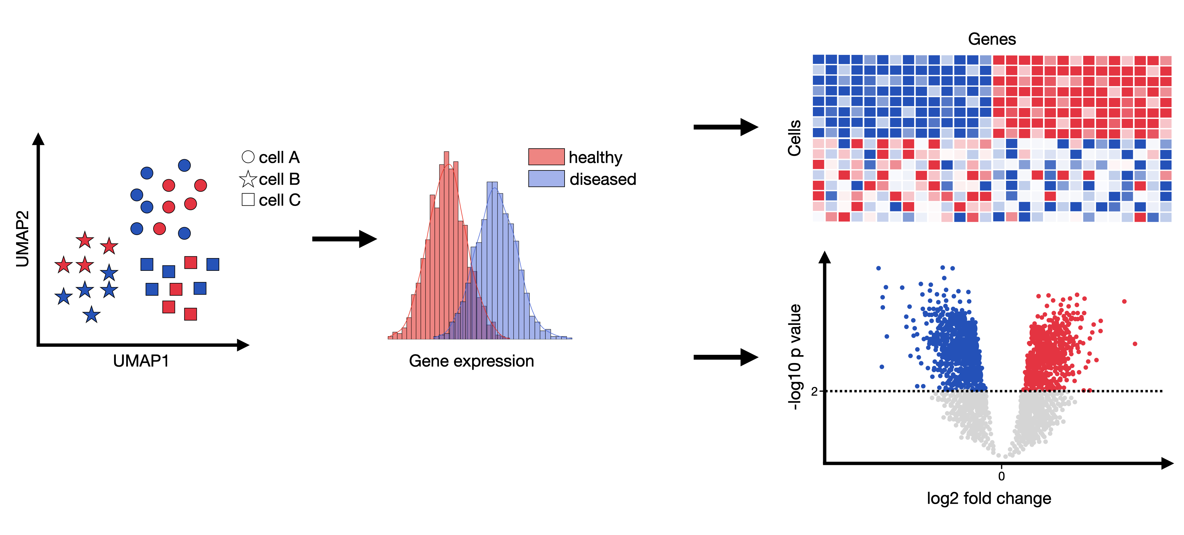
Image source: Single Cell Best Practices.
Differential gene expression analysis (DEA) attempts to infer genes that are statistically significantly over- or underexpressed between any compared groups (commonly between healthy and condition per cell type). The outcome of such an analysis could be genesets which effect and potentially explain any observed phenotypes. These genesets can then be examined more closely with respect to, for example, affected pathways or induced cell-cell communication changes.
In simple terms: DEA is a method to identify which genes are more or less active under different conditions.
Why is it important?
This analysis is crucial because it helps scientists understand how genes function in various situations. For instance, if a gene is very active in cancer cells but not in normal cells, it might be important for cancer. This understanding can lead to new treatments or a better grasp of diseases.
How does it work?
The process involves collecting data on gene expression levels from different samples. Then, statistical tests determine if the differences in expression are significant, meaning they are likely not due to random chance. This is similar to comparing test scores between two classes to see if one class performed better.
Let's break DEA down into 4 steps:
- Measure Expression: First, RNA-seq provides a snapshot of gene activity by counting how many RNA molecules (reads) correspond to each gene in the samples. This read count reflects the gene’s expression level in each sample.
- Identify Differences: DEA compares these expression levels across groups. For each gene, it assesses whether the average expression in one condition (e.g., treated) is statistically higher or lower than in the other condition (e.g., control).
- Apply Statistical Testing: To decide if the differences are meaningful, DEA uses statistical tests to see if the observed changes are likely due to the conditions rather than random variation. This analysis outputs measures like p-values and adjusted p-values (accounting for multiple testing) to indicate the significance of these changes.
- Interpret Fold-Changes: If a gene shows a large fold-change with a low p-value, it’s considered "differentially expressed" because its expression is significantly different between the conditions. These genes may then be candidates for further research, as their expression differences might reveal important biological insights about the system under study.
Note
What's a Fold-Change?
Fold change is a measure describing how much a quantity changes between an original and a subsequent measurement. It is defined as the ratio between the two quantities; for quantities A and B the fold change of B with respect to A is B/A.
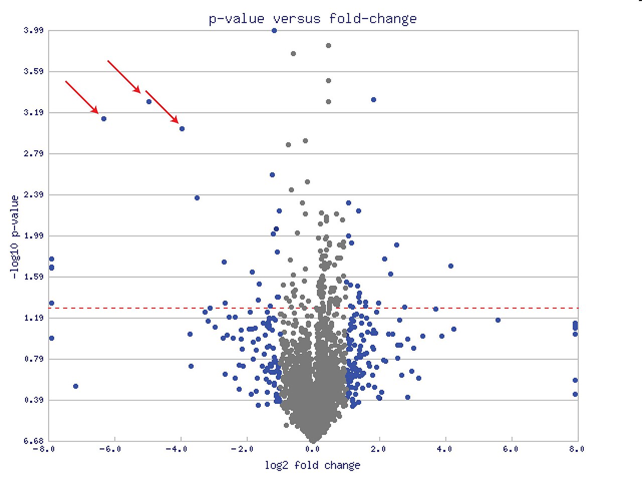
Fold-Changes are usually observed via Volcano plots, post Log2 transformation: instead of working directly with the raw fold-change, we take the logarithm (base 2) of this value. This has two main benefits:
- Symmetry: Log2 fold-change makes it easier to interpret increases and decreases equally. For example:
- A log2 fold-change of +1 means the gene expression doubled (
$2^1 = 2$ ). - A log2 fold-change of -1 means the gene expression halved (
$2^-1 = 0.5$ ).
- A log2 fold-change of +1 means the gene expression doubled (
- Range Reduction: It reduces extreme values, making data easier to handle and visualize.
Example:

In this section we discuss the steps taken prior to Differential Expression Analysis.
As mentioned above, we use the house mouse (Mus musculus, GRCm39 as model organism, and RNA-seq data obtained by Texas A&M and cleaned by us.
The tools used are:
- FastQC: quality control
- TrimGalore: trimming
- HISAT2: indexing genome, alignment to genome
- SAMtools: sorting and indexing alignment
- HTSeq: count reads in features
We have used FastQC in the past, a popular tool used to assess the quality of raw reads. The command used was:
fastqc -t 2 -o . Control1_R1.fastq.gz Control1_R2.fastq.gz
The output from FastQC was:

and

How would you interpret these readings?
Although we have not covered TrimGalore, it is tool for trimming low-quality bases and adapter sequences from high-throughput sequencing reads.
Based on the QC output above, we use TrimGalore's default settings which trims any read that is below length 20. We add the --paired option/flag to only return paired reads.
trim_galore --paired --fastqc Control1_R1.fastq.gz Control1_R2.fastq.gz
The --fastqc option/flag outputs a report we can read in FastQC.

and

Do you think TrimGalore did well? (yes).
HISAT2 is used to index the model organism of the Mouse first.
hisat2-build GCF_000001635.27_GRCm39_genomic.fna GCF_000001635.27_GRCm39_genomic
Then, HISAT2 is used to align our trimmed reads about outputting a SAM file.
 hisat2 -x GCF_000001635.27_GRCm39_genomic -p 2 -1 Control1_R1_val_1.fq.gz -2 Control1_R2_val_2.fq.gz -S Control1.sam
        .
        .
        .
236499 reads; of these:
 236499 (100.00%) were paired; of these:
30736 (13.00%) aligned concordantly 0 times
197200 (83.38%) aligned concordantly exactly 1 time
8563 (3.62%) aligned concordantly >1 times
----
30736 pairs aligned concordantly 0 times; of these:
 3583 (11.66%) aligned discordantly 1 time
----
27153 pairs aligned 0 times concordantly or discordantly; of these:
 54306 mates make up the pairs; of these:
 30660 (56.46%) aligned 0 times
 21188 (39.02%) aligned exactly 1 time
 2458 (4.53%) aligned >1 times
93.52% overall alignment rate
With 93.52% overall alignmet, we score well!
We then use SAMtools to sort our alignment and convert SAM into BAM ...
samtools sort --threads 8 \
-o Control1_sorted.bam Control1.sam
... and idex the sorted BAM file.
samtools index Control1_sorted.bam
HTSeq-count is a tool for counting the number of reads mapped to specific genomic features (like genes) in RNA-seq data.
We use flags:
-
-r pos: tells HTSeq that the reads in the BAM file are sorted by position (i.e., genomic coordinate), which can be faster if the BAM file is already sorted by position. -
-i gene: sets the feature ID attribute to use for counting ("count the genes for me please!")
htseq-count -r pos -i gene Control1_sorted.bam GCF_000001635.27_GRCm39_genomic.gff > Control1_counts.txt
We now have the data needed for DESeq2!
DESeq2 (R's Bioconductor page, BMC article by Love, Huber & Anders, 2014) is an R package widely used for analyzing RNA-seq data to identify differentially expressed genes. It takes raw read counts from sequencing data, normalizes them, performs statistical testing, and returns results that help determine which genes are significantly up- or down-regulated between conditions.
How it works
- Input Data: DESeq2 takes in raw count data for genes across samples. These counts represent the number of reads aligning to each gene in each sample.
- Normalization: DESeq2 normalizes these counts to account for factors like sequencing depth or differences between samples, ensuring a fair comparison.
- Modeling: The package models gene expression differences between conditions using a generalized linear model (GLM) and applies shrinkage to control for noise in low-expressed genes.
- Statistical Testing: DESeq2 performs statistical tests to determine if the observed changes are significant, returning metrics like the log2 fold-change and adjusted p-values for each gene.
(These are essentially the same 4 steps described above!)
Expected outputs
- Log2 fold-change: Shows the magnitude of change in gene expression between conditions. Positive values indicate up-regulation, and negative values indicate down-regulation.
- p-value: Indicates whether the observed difference is statistically significant.
- Adjusted p-value (padj): Corrects for multiple testing, helping identify genes that are reliably differentially expressed.
Quickstart (taken from the official DESeq2 guide "Analyzing RNA-seq data with DESeq2", from Love et al.)
Note
There are a variety of steps upstream of DESeq2 that result in the generation of counts or estimated counts for each sample, discussed in the above section.
Here are most basic steps for a differential expression analysis. This code chunk assumes that you have a count matrix called cts and a table of sample information called coldata. The design indicates how to model the samples, here, that we want to measure the effect of the condition, controlling for batch differences. The two factor variables batch and condition should be columns of coldata.
dds <- DESeqDataSetFromMatrix(countData = cts,
                              colData = coldata,
                              design= ~ batch + condition)
dds <- DESeq(dds)
resultsNames(dds)                                           # lists the coefficients
res <- results(dds, name="condition_trt_vs_untrt")

# or to shrink log fold changes association with condition:
res <- lfcShrink(dds, coef="condition_trt_vs_untrt", type="apeglm")
There is a variety of statements that DESeq2 uses that are different from the example above, such as using DESeqDataSetFromHTSeq() instead of DESeqDataSetFromMatrix() if you're using data from htseq-count or DESeqDataSetFromTximport() if your data is crated with Salmon.
The design parameter specifies how the experimental conditions are structured and analyzed in your RNA-seq dataset. This parameter is crucial because it tells DESeq2 which variables to use when estimating differential expression and how to model relationships between samples. Here are a few options:
- Single Factor Design: used when you have one condition or treatment group to compare, like "treated" vs. "control." (
design = ~ condition). - Two-Factor Design: used when you want to account for two independent factors, such as "condition" and "batch." (
design = ~ batch + condition). - Interaction Model: used when you have two factors and want to test if there’s an interaction between them (i.e., if the effect of one factor depends on the other) (
design = ~ condition + treatment + condition:treatment). - Multi-Factor Design: used for complex experimental setups with more than two factors, where each factor’s main effects and/or interactions are modele (
design = ~ timepoint + condition + batch).
Important
DESeq2 only creates the statistical inference. It is up to you to create the visualization plots!
Tutorial time: DESeq2 on CyVerse. We have made available an R script that will run through DESeq2 and creating PCA,volcano and heatmap plots. To get to the R script:
- Log in into CyVerse
- Go to Apps and start the JupyterLab Bioscience (8 cores min/max and 16GB memory)
- Once the App is launched, go to the Terminal:
- Do
gocmd initand login using their CyVerse credentials (username and password) - Do
gocmd get --progress /iplant/home/shared/cyverse_training/datalab/biosciences/diff-exp-analysis_tutorial/r_tutorial/
- Do
- Open RStudio and open the file using the file browser. (data-store > r_tutorial > deseq2_tut.R)
The code is runnable from beginning to end and annotated accordingly. May this be useful to you as an example in the future!
Click here for the raw code
###########################################################
# 0. LOAD NECESSARY LIBRARIES AND SET WORKING DIRECTORY  ##
###########################################################

library(ggplot2)                                          # For data visualization
library(pheatmap)                                         # For heatmap visualization
library(DESeq2)                                           # For differential gene expression analysis
library(EnhancedVolcano)                                  # For volcano plot visualization of DESeq2 results

# Set working directory
setwd("/home/jovyan/data-store/r_tutorial/counts")

###########################################################
# 1. LOADING FILES, CREATING DATASET, FILTER LOW COUNTS ###
###########################################################

# Check files in the directory
list.files()               # Lists all files in the working directory
system("cat sampleTable.csv") # Displays contents of sampleTable.csv

# Load sample table with sample metadata and conditions
sampleTable <- read.csv("sampleTable.csv", header=TRUE)   # Reads CSV file
sampleTable <- as.data.frame(sampleTable)                 # Ensures it is in data frame format
sampleTable$condition <- factor(sampleTable$condition)    # Sets 'condition' as a factor
sampleTable                                               # Displays the sample table

# Create DESeq2 dataset using counts and design information
dds <- DESeqDataSetFromHTSeqCount(sampleTable = sampleTable,
                                  directory = ".",
                                  design = ~ condition)   # Design formula for the experiment


# Show summary of DESeq2 dataset
dds

# Filter out genes with low counts across all samples
keep <- rowSums(counts(dds)) >= 10                        # Only retain genes with counts ≥ 10
dds <- dds[keep,]                                         # Updates dds to only include high-count genes

###########################################################
# 2. DIFFERENTIAL EXPRESSION ANALYSIS #####################
###########################################################

# Perform differential expression analysis
dds <- DESeq(dds)                                         # Runs DESeq2 pipeline for DE analysis
res <- results(dds)                                       # Extracts results from the DESeq2 analysis
res                                                       # Shows results with fold changes, p-values, etc.

# Count significantly differentially expressed genes
sum(res$padj <= 0.05, na.rm = TRUE)                       # Counts genes with an adjusted p-value ≤ 0.05

# Filter for significantly differentially expressed genes and save to CSV
sigGenes <- res[which(res$padj < 0.05), ]                 # Filters significant genes
write.csv(sigGenes, "Differentrially_Expressed.csv",
          row.names = TRUE)                               # Saves results

###########################################################
# 3. VISUALIZATION: #######################################
#   3.1 PCA PLOT    #######################################
###########################################################

# Regularized log transformation to stabilize variance
logTran <- rlog(dds)

# Calculate row variances and select top variable genes
rv <- rowVars(assay(logTran))                             # Calculates variance for each gene across samples
select <- order(rv, decreasing = TRUE)[seq_len(min(100, length(rv)))] # Selects top 100 variable genes

# Perform Principal Component Analysis (PCA) on selected genes
PCA <- prcomp(t(assay(logTran)[select, ]), scale = FALSE) # Runs PCA
summary(PCA)                                              # Shows PCA summary

# Calculate and prepare variance explained for plotting
percentVar <- round(100*PCA$sdev^2/sum(PCA$sdev^2), 1)    # Calculates percent variance for each PC
ggPCA_out <- as.data.frame(PCA$x)                         # Converts PCA output to data frame
ggPCA_out <- cbind(ggPCA_out, sampleTable)                # Adds sample information to PCA data

# Plot PCA with ggplot2
ggplot(ggPCA_out, aes(x=PC1, y=PC2, color=condition)) +
  geom_point(size=4) +
  labs(x = paste0("PC1 - variance explained: ", percentVar[1], "%"),
       y = paste0("PC2 - variance explained: ", percentVar[2], "%")) +
  theme_bw()                                              # Adds basic theme

###########################################################
# 3. VISUALIZATION:  ######################################
#   3.2 VOLCANO PLOT ######################################
###########################################################

# Create volcano plot for differential expression results
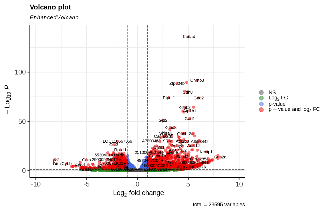
EnhancedVolcano(res,
                lab = rownames(res),
                x = 'log2FoldChange',
                y = 'padj',
                pCutoff = 0.05,                          # Significance threshold
                FCcutoff = 1.0,                          # Fold-change threshold
                pointSize = 3.0,                         # Point size
                labSize = 4.0,                           # Label size
                colAlpha = 1/2,                          # Point transparency
                drawConnectors = FALSE,                  # Disable connectors for labels
                legendPosition = "right")                # Position legend

##########################################################
# 3. VISUALIZATION:  #####################################
#   3.3 HEATMAP      #####################################
##########################################################


# Filter top significant genes with strong log2 fold-change for heatmap
resorted_deresults <- res[order(res$padj),]              # Sort results by adjusted p-value
sig <- resorted_deresults[!is.na(resorted_deresults$padj) &
                            resorted_deresults$padj < 0.05 &
                            abs(resorted_deresults$log2FoldChange) >= 6.5, ]

selected <- rownames(sig)                                # Get names of selected genes
selected                                                 # Display selected genes

# Plot heatmap of selected gene expression values
transformed_readcounts <- normTransform(dds)             # Apply variance-stabilizing transformation
pheatmap(assay(transformed_readcounts)[selected,],
         cluster_rows = TRUE, show_rownames = TRUE,
         cluster_cols = TRUE,
         labels_col = colData(dds)$sampleName)           # Plots heatmap with clustering of samples and genes
- The official DESeq2 tutorial on Bioconductor
- The DESeq2 paper by Love, Huber & Anders, BMC, 2014
- "Beginner's guide to using the DESeq2 package" by Love, Anders & Huber (not really for beginners, but hey, they tried)
- An advanced tutorial on DEA by Single Cell Best Practices using Python
UArizona DataLab, Data Science Institute, University of Arizona, 2024.