Implementation of piecewise structural equation modeling (SEM) in R, including estimation of path coefficients and goodness-of-fit statistics.
A formal description of this package can be found at:
Lefcheck, Jonathan S. (2015) piecewiseSEM: Piecewise structural equation modeling in R for ecology, evolution, and systematics. Methods in Ecology and Evolution. 7(5): 573-579. DOI: 10.1111/2041-210X.12512
Version: 1.2.1 (2016-12-06)
Author: Jon Lefcheck [email protected]
Supported model classes include:
lm, glm, rq, glm.nb, gls, pgls, merMod, merModLmerTest, lme, glmmPQL, glmmadmb, and glmmTMB.
###WARNING
Some tests of directed separation are non-symmetrical -- the partial slope of a ~ b is not the same as b ~ a -- when the variables are non-linear (i.e., are transformed via a link function when fit to a non-normal distribution). We are currently investigating the phenomenon, but in the interim, the latest version of the package returns the lowest P-value. This the more conservative route. Stay tuned for more updates...
This is only a problem if you are fitting generalized linear models!!
##Examples
###Load package
# Install latest version from CRAN
install.packages("piecewiseSEM")

# Install dev version from GitHub
# library(devtools)
# install_github("jslefche/piecewiseSEM")

library(piecewiseSEM)
###Load data from Shipley 2009
data(shipley2009)
The data is alternately hosted in Ecological Archives E090-028-S1 (DOI: 10.1890/08-1034.1).
###Create model set
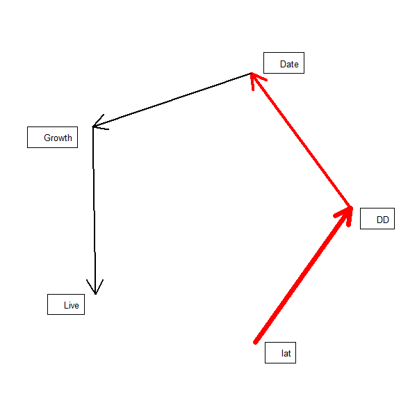
The model corresponds to the following hypothesis (Fig. 2, Shipley 2009);
Models are constructed using a mix of the nlme and lmerTest packages, as in the supplements of Shipley 2009.
# Load required libraries for linear mixed effects models
library(lme4)
library(nlme)

# Load example data
data(shipley2009)

# Create list of models corresponding to SEM
shipley2009.modlist = list(

  lme(DD~lat, random = ~1|site/tree, na.action = na.omit,
  data = shipley2009),

  lme(Date~DD, random = ~1|site/tree, na.action = na.omit,
  data = shipley2009),

  lme(Growth~Date, random = ~1|site/tree, na.action = na.omit,
  data = shipley2009),

  glmer(Live~Growth+(1|site)+(1|tree),
  family=binomial(link = "logit"), data = shipley2009)

  )
###Run Shipley tests
sem.fit returns a list of the following:
(1) the missing paths (omitting conditional variables), the estimate, standard error, degrees of freedom, and associated p-values;
(2) the Fisher's C statistic, degrees of freedom, and p-value for the model (derived from a Chi-squared distribution);
(3) the AIC, AICc (corrected for small sample size), the likelihood degrees of freedom, and the model degrees of freedom.
The argument add.vars allows you to specify a vector of additional variables whose causal independence you also wish to test. This is useful if you are comparing nested models. Default is NULL.
The argument adjust.p allows you to adjust the p-values returned by the function based on the the total degrees of freedom for the model (see supplementary material, Shipley 2013). Default is FALSE (uses the d.f. reported in the summary table).
(See "p-values and all that" for a discussion of p-values from mixed models using the lmer package.)
sem.fit(shipley2009.modlist, shipley2009)

# Conditional variables have been omitted from output table for clarity (or use argument conditional = T)
# $missing.paths
#         missing.path estimate std.error   df crit.value p.value
# 1   Date ~ lat + ...  -0.0091    0.1135   18    -0.0798  0.9373
# 2 Growth ~ lat + ...  -0.0989    0.1107   18    -0.8929  0.3837
# 3   Live ~ lat + ...   0.0305    0.0297   NA     1.0279  0.3040
# 4  Growth ~ DD + ...  -0.0106    0.0358 1329    -0.2967  0.7667
# 5    Live ~ DD + ...   0.0272    0.0271   NA     1.0046  0.3151
# 6  Live ~ Date + ...  -0.0466    0.0298   NA    -1.5622  0.1182
#
# $Fisher.C
#   fisher.c df p.value
# 1    11.54 12   0.483
#
# $AIC
#     AIC   AICc  K    n
# 1 49.54 50.079 19 1431
The missing paths output differs from Table 2 in Shipley 2009. However, running each d-sep model by hand yields the same answers as this function, leading me to believe that updates to the lme4 and nlme packages are the cause of the discrepancy. Qualitatively, the interpretations are the same.
###Extract path coefficients
Path coefficients can be either unstandardized or standardized (centered and scaled in units of standard deviation of the mean, or scaled by the range the data). Default is none. The function returns a data.frame sorted by increasing significance.
sem.coefs(shipley2009.modlist, shipley2009)

#   response predictor   estimate   std.error p.value
# 1       DD       lat -0.8354736 0.119422385       0 ***
# 2     Date        DD -0.4976475 0.004933274       0 ***
# 3   Growth      Date  0.3007147 0.026631405       0 ***
# 4     Live    Growth  0.3478536 0.058415948       0 ***

sem.coefs(shipley2009.modlist, shipley2009, standardize = "scale")

#   response predictor   estimate   std.error p.value
# 1       DD       lat -0.7014051 0.100258794       0 ***
# 2     Date        DD -0.6281367 0.006226838       0 ***
# 3   Growth      Date  0.3824224 0.033867469       0 ***
# 4     Live    Growth  0.3478536 0.058415948       0 ***
# Warning message:
# In get.scaled.data(modelList, data, standardize) :
#   One or more responses not modeled to a normal distribution: keeping response(s) on original scale!
Note the error indicating that one of the responses (Live) cannot be scaled because it would violate the distributional assumptions, so only the predictors have been scaled.
We can plot a rudimentary path diagram of the SEM using sem.plot which reports the coefficients, above:
sem.plot(shipley2009.modlist, shipley2009)
###Generate variance-covariance SEM using lavaan
Generate variance-covariance based SEM from the list of linear mixed models. The resulting object can be treated like any other model object constructed using the package lavaan.
(lavaan.model = sem.lavaan(shipley2009.modlist, shipley2009))

# lavaan (0.5-18) converged normally after  27 iterations
#
#                                                   Used       Total
#   Number of observations                          1431        1900
#
#   Estimator                                         ML
#   Minimum Function Test Statistic               38.433
#   Degrees of freedom                                 6
#   P-value (Chi-square)                           0.000
The output shows that the variance-covariance SEM is a worse fit, indicating that a hierarchical piecewise approach is justified given the hierarchical structure of the data.
###Plot partial effect between two variables
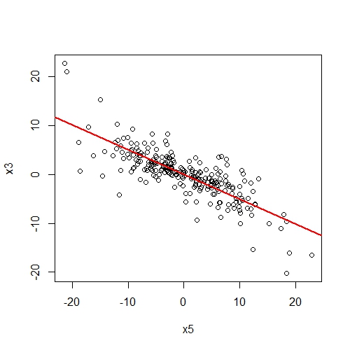
One might be interested in the partial effects of one variable on another given covariates in the SEM. The function partial.resid returns a data.frame of the partial residuals of y ~ x and plots the partial effect (if plotit = T).
# Load model package
library(nlme)

# Load data from Shipley (2013)
data(shipley2013)

# Create list of structured equations
shipley2013.modlist = list(

  lme(x2~x1, random = ~x1 | species, data = shipley2013),

  lme(x3~x2, random = ~x2 | species, data = shipley2013),

  lme(x4~x2, random = ~x2 | species, data = shipley2013),

  lme(x5~x3+x4, random = ~x3+x4 | species, data = shipley2013)

  )

# Get partial residuals of x3 on x5 conditional on x4
resids.df = partial.resid(x5 ~ x3, shipley2013.modlist, list(lmeControl(opt = "optim")))
###Get R2 for individual models
Return R2 and AIC values for component models in the SEM.
sem.model.fits(shipley2009.modlist)

#      Class   Family     Link    N  Marginal Conditional
# 1      lme gaussian identity 1431 0.4766448   0.6932571
# 2      lme gaussian identity 1431 0.4083328   0.9838487
# 3      lme gaussian identity 1431 0.1070265   0.8364736
# 4 glmerMod binomial    logit 1431 0.5589205   0.6291980
###Return model predictions
Generate model predictions from new data.
# Create new data for predictions
shipley2009.new = data.frame(

  lat = rnorm(length(shipley2009$lat), mean(shipley2009$lat, na.rm = T),
    sd(shipley2009$lat, na.rm = T)),

  DD = rnorm(length(shipley2009$DD), mean(shipley2009$DD, na.rm = T),
    sd(shipley2009$DD, na.rm = T)),

  Date = rnorm(length(shipley2009$Date), mean(shipley2009$Date, na.rm = T),
    sd(shipley2009$Date, na.rm = T)),

  Growth = rnorm(length(shipley2009$Growth), mean(shipley2009$Growth, na.rm = T),
    sd(shipley2009$Growth, na.rm = T))

)

# Generate predictions
head(sem.predict(shipley2009.modlist, shipley2009.new))


