Overview of Deep Learning Algorithms

What is Deep Learning?

Image Credit: TowardsAI.net

---

From Wikipedia:

Deep learning is part of a broader family of machine learning methods based on artificial neural networks with representation learning. Learning can be supervised, semi-supervised or unsupervised.

Deep-learning architectures such as deep neural networks, deep belief networks, deep reinforcement learning, recurrent neural networks, convolutional neural networks and Transformers have been applied to fields including computer vision, speech recognition, natural language processing, machine translation, bioinformatics, drug design, medical image analysis, climate science, and board game programs, where they have produced results comparable to and in some cases surpassing human expert performance.

Image credit: Sam Greydanus.

What is the difference between Machine Learning and Deep Learning?

Image Credit: TowardsAI.net

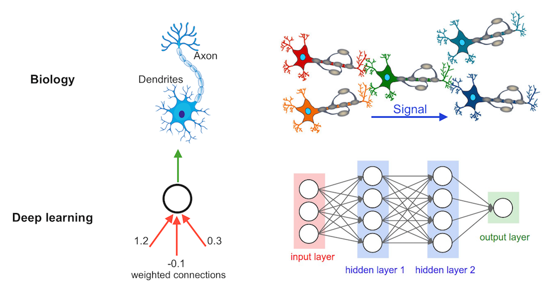
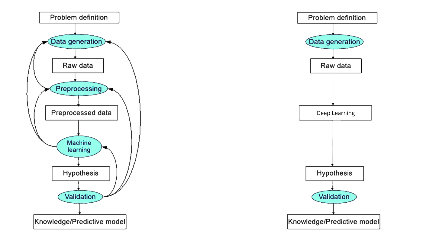
The process of training a model in Deep Learning is directly inputting the data into the model. The model will learn and perform the classification.

Single Layer Neural Network

Image credit: Sebastian Raschka

At a basic level, a neural network is comprised of four main components: inputs, weights, a bias (or threshold or intercept), and an output. Similar to linear regression, the algebraic formula would look something like this:

$$ \hat{y} = \sum_{i=1}^{m} w_{i} x_{i} + bias = w_{0} + w_{1} x_{1} + w_{2} x_{2} + \ldots + w_{m} x_{m} $$

The above equation for the prediction value $\hat{y}$ can be expressed as a dot product of a weight vector $\vec{w} \in R^{d}$ and a feature vector $\vec{x} \in R^{d}$ plus some bias or intercept $b$. Both $\vec{w}$ and $\vec{x}$ are elements of a real $d$-dimensional space.

$$ \hat{y} = \vec{w}^{T} \vec{x} + b $$

---

Example: Whether or not you should order a pizza for dinner. This will be our predicted outcome, or $\hat{y}$.

Let’s assume that there are three main factors that will influence your decision:

• If you will save time by ordering out (Yes: 1; No: 0)
• If you will lose weight by ordering a pizza (Yes: 1; No: 0)
• If you will save money (Yes: 1; No: 0)

Then, let’s assume the following, giving us the following inputs:

• $x_1 = 1$, since you’re not making dinner
• $x_2 = 0$, since we’re getting ALL the toppings
• $x_3 = 1$, since we’re only getting 2 slices

For simplicity purposes, our inputs will have a binary value of 0 or 1. This technically defines it as a perceptron as neural networks primarily leverage sigmoid neurons.

Next need to assign some weights to determine importance. Larger weights make a single input’s contribution to the output more significant compared to other inputs.

• $w_1 = 5$, since you value time
• $w_2 = 3$, since you value staying in shape
• $w_3 = 2$, since you've got money in the bank

Finally, we’ll also assume a threshold value of 5, which would translate to a bias value of –5.

Using the following activation function, we can now calculate the output (i.e., our decision to order pizza):

$$ {\rm output}: \ \ \ f(x) = 1 \ \ if \ \ \hat{y} \ge 0 \ \ \ else \ \ \ f(x) = 0 \\ $$

In summary:

$\hat{y}$ (our predicted outcome) = Decide to order pizza or not

$$ \begin{eqnarray} \hat{y} & = & (5 * 1) + (3 * 0) + (2 * 1) - 5 \\ & = & 5 + 0 + 2 – 5 \\ & = & 2 \\ \end{eqnarray} $$

Since $\hat{y}$ is 2, the output from the activation function will be 1, meaning that we will order pizza.

---

Loss function

Loss functions quantify the distance between the real and predicted values of the target. The loss will usually be a non-negative number where smaller values are better and perfect predictions incur a loss of 0. For regression problems, the most common loss function is squared error.

Image Credit: d2l.ai

When we measure the loss as a sum of squares of the differences, we may end up with large quantities, especially when there are some outlier data. To measure the quality of a model on the entire dataset of $n$ examples, we simply average (or equivalently, sum) the losses on the training set:

$$ \begin{eqnarray} L(\vec{w},b) & = & \frac{1}{n} \sum_{i=1}^{n} l^{(i)} (\vec{w},b) \\ & = & \frac{1}{n} \sum_{i=}^{n} \frac{1}{2} ( \vec{w}^{T} \vec{x}^{(i)} + b - y^{(i)} )^{2} \\ \end{eqnarray} $$

When training the model, we want to find the optimal parameters $(\vec{w}^{∗},b^{*})$ that minimize the total loss across all training examples.

Stochastic Gradient Descent

The key technique for optimizing nearly any deep learning model consists of iteratively reducing the error by updating the parameters in a direction that incrementally lowers the loss function. This algorithm is called stochastic gradient descent.

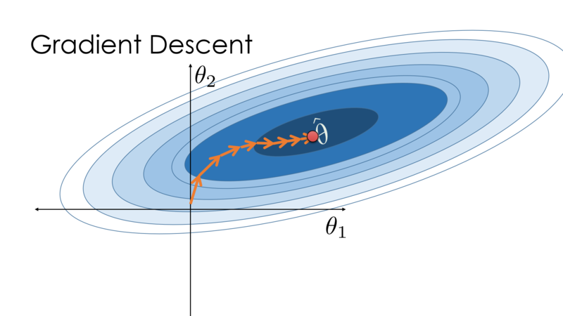
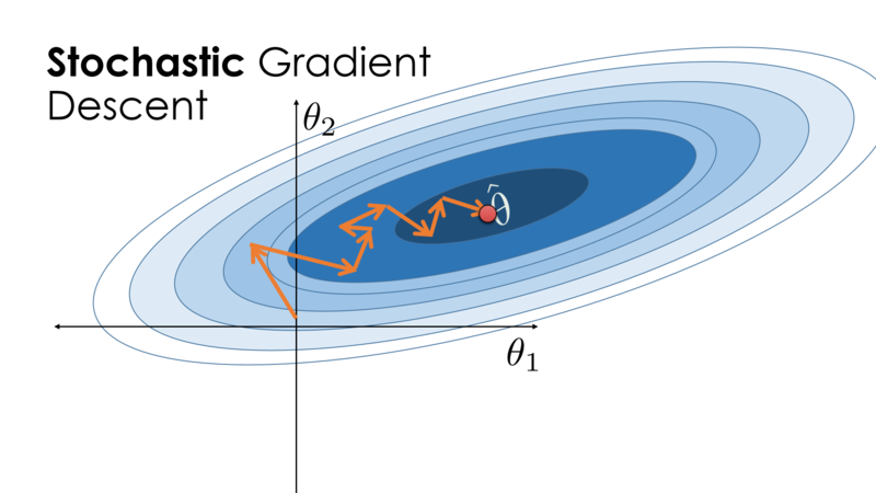
Image Credit: Cornell's University Computational Optimization Textbook

Multi-layer Neural Network

Image credit: Sebastian Raschka

The simplest deep networks are called multilayer perceptrons, and they consist of multiple layers of neurons each fully connected to those in the layer below (from which they receive input) and those above (which they, in turn, influence).

Let's exemplify with a neural network with L=3 layers.

Image credit: Sebastian Raschka

From Linear to Nonlinear Equations

The above model with m=3 input variables (3 variables with $n$ observations each), 1 hidden layer with d=4 hidden units, and t=3 output units.

If $\vec{X} \in R^{n \times m}$ represents the input variable, with a weight vector $\vec{W}^{(1)} \in R^{m \times d}$ and bias $b^{(1)} \in R^{1 \times d}$, then this 3 layers neural network model can be described by the set of equations

$$ \begin{eqnarray} \vec{H} & = & \vec{X} \vec{W}^{(1)} + b^{(1)} \\ \vec{O} & = & \vec{H} \vec{W}^{(2)} + b^{(2)} \\ \end{eqnarray} $$

where $\vec{H} \in R^{n \times d}$ are the values of the variables in the hidden layer, with a corresponding weight vector $\vec{W}^{(2)}\in R^{d \times t}$ and bias $b^{(2)} \in R^{1 \times t}$.

The prediction of the model is given by the output vector $\vec{O} \in R^{n \times t}$.

Activation Functions

In order to realize the potential of multilayer architectures, we need one more key ingredient: a nonlinear activation function $σ$ to be applied to each hidden unit following the affine transformation. For instance, a popular choice is the ReLU (Rectified Linear Unit) activation function $σ(x) = max(0,x)$ operating on its arguments element-wise. The outputs of activation functions $σ(⋅)$ are called activations. In general, with activation functions in place, it is no longer possible to collapse our multilayer neural network into a linear model:

$$ \begin{eqnarray} \vec{H} & = & \sigma (\vec{X} \vec{W}^{(1)} + b^{(1)}) \\ \vec{O} & = & \vec{H} \vec{W}^{(2)} + b^{(2)} \\ \end{eqnarray} $$

To build more general multilayer neural networks, we can continue stacking such hidden layers, e.g., $\vec{H}^{(1)} = \sigma_1 (\vec{X} \vec{W}^{(1)} + b^{(1)})$ and $\vec{H}^{(2)} = \sigma_2 (\vec{H}^{(1)} \vec{W}^{(2)} + b^{(2)})$, one atop another, yielding ever more expressive models.

There is no definitive guide for which activation function works best on specific problems. It’s a trial and error process where one should try a different set of functions and see which one works best on the problem at hand.

There are several options for selecting activation functions:

• Rectified Linear Unit (ReLU):

$$ ReLU(x) = \max(0,x) $$

Image credit: d2l.ai

• The sigmoid function transforms its inputs, for which values lie in the domain R, to outputs that lie on the interval (0, 1):

$$ sigmoid = \frac{1}{1 + \exp(-x)} $$

Image credit: d2l.ai

• Like the sigmoid function, the tanh (hyperbolic tangent) function also squashes its inputs, transforming them into elements on the interval between -1 and 1:

$$ \tanh(x) = \frac{1 - \exp(-2x)}{1 + \exp(-2x)} $$

Image credit: d2l.ai

Forward & Backward propagation

The input $\vec{X}$ provides the initial information that then propagates to the hidden units at each layer and finally produces the output $\hat{y}$.

The architecture of the network entails determining its depth, width, and activation functions used on each layer. Depth is the number of hidden layers. Width is the number of units (nodes) on each hidden layer since we don’t control either the input layer or output layer dimensions.

Research has proven that deeper networks outperform networks with more hidden units. Therefore, it’s always better and won’t hurt to train a deeper network.

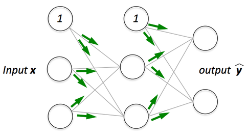
If we have a multi-layer neural network, we can picture forward propagation (passing the input signal through a network while multiplying it by the respective weights to compute an output) as follows:

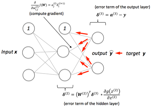
And in backpropagation, we “simply” backpropagate the error (the “cost” that we compute by comparing the calculated output and the known, correct target output, which we then use to update the model parameters):

Images credit: Sebastian Raschka

Neural Network Types

Image credit: Fjodor Van Veen

Feedforward neural networks (FF or FFNN) and perceptrons (P)

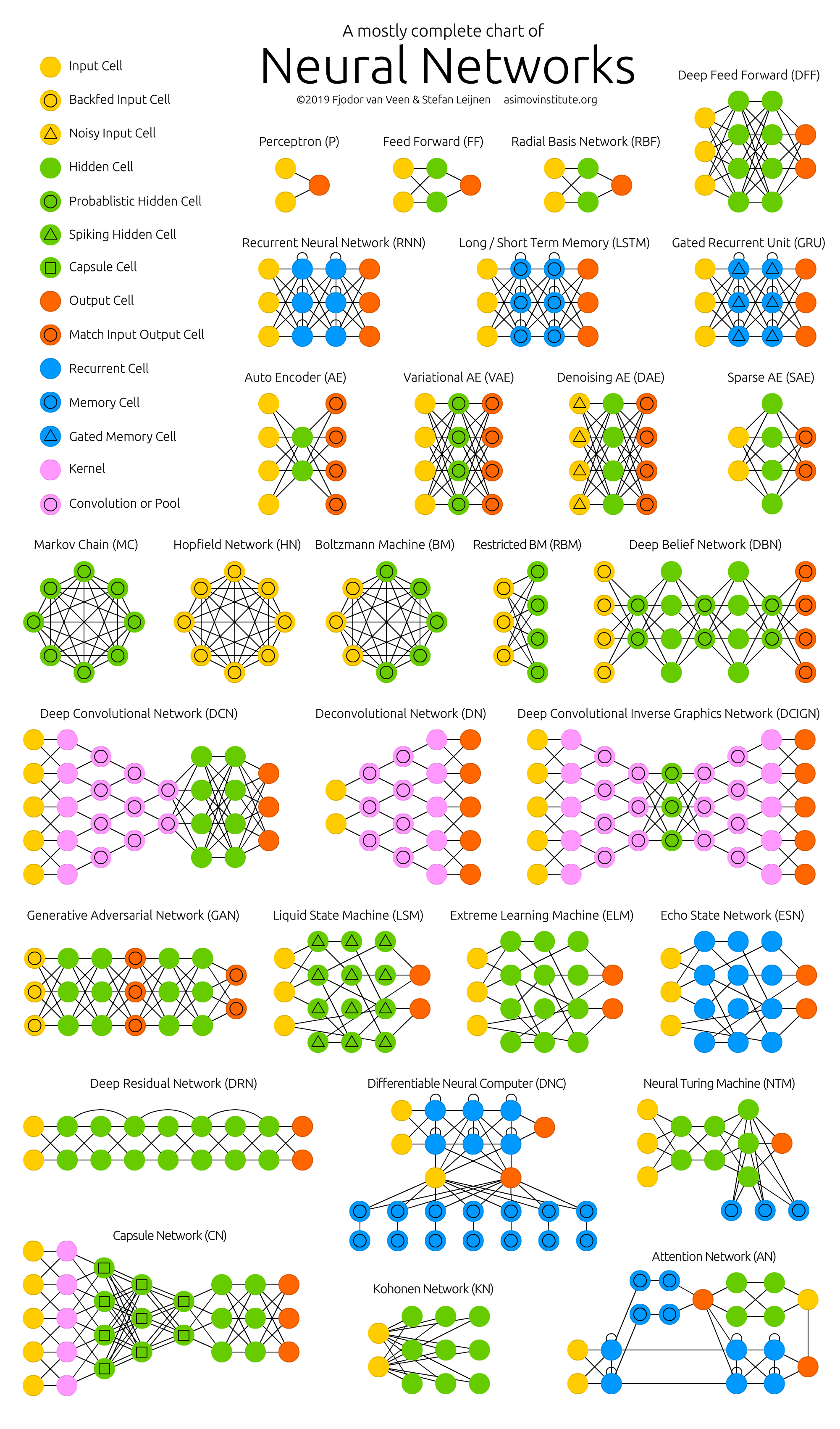
A feedforward neural network is an artificial neural network wherein connections between the nodes do not form a cycle. As such, it is different from its descendant: recurrent neural networks. The feedforward neural network was the first and simplest type of artificial neural network devised.

Radial Basis Function (RBF)

The popular type of feed-forward network is the radial basis function (RBF) network. It has two layers, not counting the input layer, and contrasts from a multilayer perceptron in the method that the hidden units implement computations.

Recurrent neural networks (RNN)

A recurrent neural network is a class of artificial neural networks where connections between nodes can create a cycle, allowing output from some nodes to affect subsequent input to the same nodes. This allows it to exhibit temporal dynamic behavior.

Long / short term memory (LSTM)

Long short-term memory is an artificial neural network used in the fields of artificial intelligence and deep learning. Unlike standard feedforward neural networks, LSTM has feedback connections. Such a recurrent neural network can process not only single data points, but also entire sequences of data.

Gated recurrent units (GRU)

A gated recurrent unit (GRU) is a gating mechanism in recurrent neural networks (RNN) similar to a long short-term memory (LSTM) unit but without an output gate. GRU's try to solve the vanishing gradient problem that can come with standard recurrent neural networks.

Bidirectional recurrent neural networks, bidirectional long / short term memory networks and bidirectional gated recurrent units (BiRNN, BiLSTM and BiGRU respectively)

Bidirectional recurrent neural networks connect two hidden layers of opposite directions to the same output. With this form of generative deep learning, the output layer can get information from past and future states simultaneously.

Autoencoders (AE)

An autoencoder is a type of artificial neural network used to learn efficient codings of unlabeled data. The encoding is validated and refined by attempting to regenerate the input from the encoding. The autoencoder learns a representation for a set of data, typically for dimensionality reduction, by training the network to ignore insignificant data.

Variational autoencoders (VAE)

In machine learning, a variational autoencoder, is an artificial neural network architecture introduced by Diederik P. Kingma and Max Welling, belonging to the families of probabilistic graphical models and variational Bayesian methods.

Denoising autoencoders (DAE)

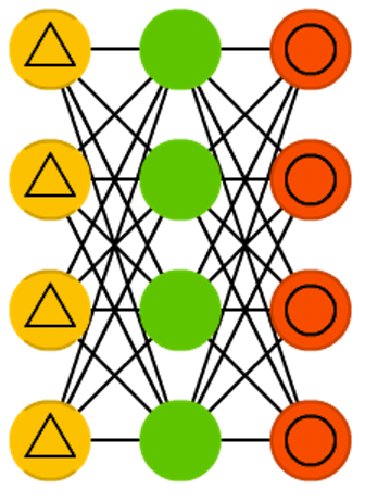
The Denoising Autoencoder (DAE) approach is based on the addition of noise to the input image to corrupt the data and to mask some of the values, which is followed by image reconstruction.

Sparse autoencoders (SAE)

A sparse autoencoder is one of a range of types of autoencoder artificial neural networks that work on the principle of unsupervised machine learning. Autoencoders are a type of deep network that can be used for dimensionality reduction – and to reconstruct a model through backpropagation.

Markov chains (MC or discrete time Markov Chain, DTMC)

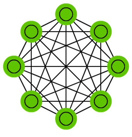
In probability, a Markov chain is a sequence of random variables, known as a stochastic process, in which the value of the next variable depends only on the value of the current variable, and not any variables in the past. For instance, a machine may have two states, A and E.

Hopfield network (HN)

A Hopfield network is a form of recurrent artificial neural network and a type of spin glass system popularised by John Hopfield in 1982 as described earlier by Little in 1974 based on Ernst Ising's work with Wilhelm Lenz on the Ising model.

Boltzmann machines (BM)

A Boltzmann machine is a stochastic spin-glass model with an external field, i.e., a Sherrington–Kirkpatrick model, that is a stochastic Ising Model. It is a statistical physics technique applied in the context of cognitive science. It is also classified as Markov random field.

Restricted Boltzmann machines (RBM)

A restricted Boltzmann machine is a generative stochastic artificial neural network that can learn a probability distribution over its set of inputs. RBMs were initially invented under the name Harmonium by Paul Smolensky in 1986, and rose to prominence after Geoffrey Hinton and collaborators invented fast learning algorithms for them in the mid-2000.

Deep belief networks (DBN)

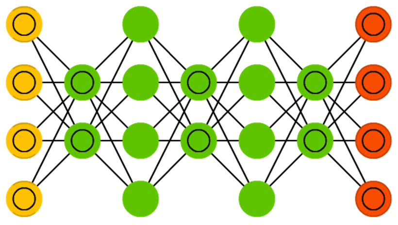
In machine learning, a deep belief network is a generative graphical model, or alternatively a class of deep neural network, composed of multiple layers of latent variables, with connections between the layers but not between units within each layer.

Convolutional neural networks (CNN or deep convolutional neural networks, DCNN)

In deep learning, a convolutional neural network is a class of artificial neural network, most commonly applied to analyze visual imagery. CNNs are also known as Shift Invariant or Space Invariant Artificial Neural Networks, based on the shared-weight architecture of the convolution kernels or filters that slide along input features and provide translation-equivariant responses known as feature maps.

Deconvolutional networks (DN)

[Deconvolutional networks](https://www.techopedia.com/definition/33290/deconvolutional-neural-network-dnn are convolutional neural networks (CNN) that work in a reversed process. Deconvolutional networks, also known as deconvolutional neural networks, are very similar in nature to CNNs run in reverse but are a distinct application of artificial intelligence.

Deep convolutional inverse graphics networks (DCIGN)

The deep convolutional inverse graphics network (DC-IGN) is a particular type of convolutional neural network that is aimed at relating graphics representations to images. Experts explain that a deep convolutional inverse graphics network uses a “vision as inverse graphics” paradigm that uses elements like lighting, object location, texture and other aspects of image design for very sophisticated image processing.

Generative adversarial networks (GAN)

A generative adversarial network is a class of machine learning frameworks designed by Ian Goodfellow and his colleagues in June 2014. Two neural networks contest with each other in the form of a zero-sum game, where one agent's gain is another agent's loss.

Liquid state machines (LSM)

A liquid state machine is a type of reservoir computer that uses a spiking neural network. An LSM consists of a large collection of units. Each node receives time varying input from external sources as well as from other nodes. Nodes are randomly connected to each other.

Extreme learning machines (ELM)

Most commonly used Deep Learning Libraries

Image credit: zhuanlan.Zhihu.com

There is a wide variety of deep learning libraries, but currently, you will find that many applications use one of the following:

• Tensorflow developed by Google Brain,
• Keras, a user-friendly framework that works on top of Tensorflow 2.0.
• Pytorch developed originally by Meta AI and now under the umbrella of the Linux Foundation, and
• Apache MXNet.

Tensorflow

The latest version is Tensorflow 2.0.

You can find all the Tensorflow documentation and learning resources in this link.

More Tensorflow resources:

• Models and datasets
• Tools
• Libraries extensions
• Responsible AI
• Tensorflow Github Repo

Pytorch

The latest version is Pytorch 1.13.

You can find the Pytorch Learning Resources in this link.

More Pytorch resources:

• Getting started
• Documentation
• Resources
• Pytorch Github Repo

Apache MXNet

The latest version is MXNet 1.9.1.

More Apache MXNet resources:

• Getting started
• Documentation and Tutorials
• Apache MXNet Github Repo

---

References

• Deep Learning. Wikipedia.
• Deep Learning. IBM Cloud Education.
• A Visual and Interactive Guide to the Basics of Neural Networks. Jay Alammar.
• The Neural Network Zoo. Fjodor Van Veen, The Asimov Institute.
• Three Perspectives on Deep Learning. Sam Greydanus.
• Dive into Deep Learning. Aston Zhang, Zachary C. Lipton, Mu Li, and Alexander J. Smola.
• Python Machine Learning, 3rd. Ed., Sebastian Raschka, and Vahid Mirjalili.
• The Principles of Deep Learning Theory. Roberts, Daniel A. and Yaida, Sho and Hanin, Boris.

Cheat Sheets

• CS-229 Machine Learning. Shervine Amidi, Stanford University; Afshine Amidi, MIT.
• CS-230 Deep Learning. Shervine Amidi, Stanford University; Afshine Amidi, MIT.

---

Created: 11/25/2022

Updated: 11/29/2022

Carlos Lizárraga

CC BY-NC-SA

The University of Arizona. Data Science Institute, 2022.