Introduction to Time Series Analysis

Time Series

In mathematics, a time series is a series of data points indexed in time order. Most commonly, a time series is a sequence taken at successive equally spaced points in time. Thus it is a sequence of discrete-time data. Examples of time series are heights of ocean tides, counts of sunspots, and the daily closing value of the Dow Jones Industrial Average.

A time series is very frequently plotted via a run chart (which is a temporal line chart). Time series are used in statistics, signal processing, pattern recognition, econometrics, mathematical finance, weather forecasting, earthquake prediction, electroencephalography, control engineering, astronomy, communications engineering, and largely in any domain of applied science and engineering which involves temporal measurements.

Time series analysis comprises methods for analyzing time series data in order to extract meaningful statistics and other characteristics of the data. Time series forecasting is the use of a model to predict future values based on previously observed values.

Time series analysis and forecasting is a branch of statistics that deals with analyzing and predicting the patterns and trends in time series data.

Some of the main topics in time series analysis and forecasting include:

Time series data: This topic covers the different types of time series data and how to collect, organize, and visualize them.
Time domain analysis: This topic covers the basic time domain techniques such as trend analysis, seasonality, and cyclical patterns.
Frequency domain analysis: This topic covers the Fourier analysis and other frequency domain techniques to explore and extract the hidden periodicities in time series data.
Stationarity and non-stationarity: This topic covers the concepts of stationarity, non-stationarity, and how to test and transform time series data to meet the stationarity assumption.
Autocorrelation and cross-correlation: This topic covers the concepts of autocorrelation and cross-correlation functions and how to use them to detect and measure the relationship between lagged values of a time series.
Time series models: This topic covers the different types of time series models such as ARIMA, Seasonal ARIMA, and exponential smoothing models and how to estimate and diagnose them.
Forecasting: This topic covers the various methods and techniques used for forecasting future values of a time series, such as ARIMA, exponential smoothing, and neural network models.
Model selection and validation: This topic covers the methods and techniques for selecting the best time series model for a particular data set and how to validate the performance of the selected model.
Multivariate time series analysis: This topic covers the analysis of time series data that involve multiple variables, such as VAR and VECM models.

Overall, time series analysis and forecasting is a vast and important area of study that has many practical applications in fields such as economics, finance, engineering, and environmental sciences.

Best-known Python libraries for Time Series Analysis

There are several Python libraries available for Time Series Analysis. Here are some of the most popular ones:

Statsmodels is a general-purpose statistics library that includes modules for time series analysis. (statsmodels.tsa, statsmodels.tsa.arima.model.ARIMA)
Pandas is a data analysis library that includes a module for time series analysis.
Scikit-learn is a machine learning library that includes a module for [time series analysis].
sktime is a library for time series analysis in Python. It provides a unified interface for multiple time series learning tasks. Currently, this includes time series classification, regression, clustering, annotation, and forecasting. It comes with time series algorithms and scikit-learn compatible tools to build, tune and validate time series models.
pmdarima (originally pyramid-Arima, for the anagram of 'py' + 'Arima') is a statistical library designed to fill the void in Python's time series analysis capabilities. Pmdarima wraps statsmodels under the hood, but is designed with an interface that's familiar to users coming from a scikit-learn background.
tsfresh (Time Series Feature extraction based on scalable hypothesis tests), the package provides systematic time-series feature extraction by combining established algorithms from statistics, time-series analysis, signal processing, and nonlinear dynamics with a robust feature selection algorithm.
PyFlux is a time series analysis library specifically designed for forecasting.
TensorFlow is a machine learning library that includes a module for time series analysis.
Prophet: This is a forecasting library developed by Facebook that provides tools for time-series analysis and forecasting. It has several built-in models for trend analysis, seasonality, and growth, as well as functions for time-series visualization.
statsforecast offers a collection of popular univariate time series forecasting models optimized for high performance and scalability.

These libraries offer a variety of features for time series analysis, including:

Data import and export
Data cleaning and preprocessing
Time series modeling
Time series forecasting
Time series visualization

The choice of which library to use will depend on the specific needs of the project. For example, if the project requires a lot of data cleaning and preprocessing, then Pandas or Scikit-learn may be a good choice. If the project involves a lot of time series modeling and forecasting, then PyFlux or TensorFlow may be a good choice.

There are many other libraries available for time-series analysis in Python, but these are some of the most popular and widely used ones.

Components of a Time Series

Before we begin describing time series, we describe a list of basic concepts:

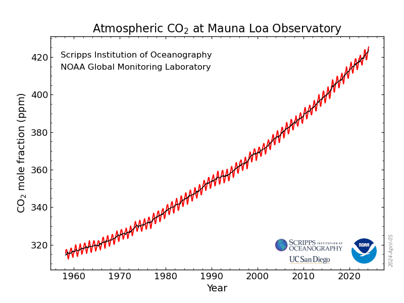
Trend: It refers to whether data values increase or decrease with time.

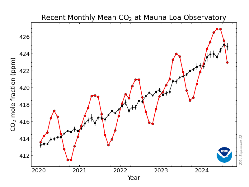
Seasonality and cycles: Seasonality is a repeated behavior of data that occurs on the regular interval of time. It means that there are patterns that repeat themselves after some interval of the period then we call it seasonality.

The difference between seasonality and cycles is that seasonality is always has a fixed and a known frequency. The cycles also have rise and fall peaks but not a fixed frequency. The Solar cycle duration is nearly 11 years.

Variations and Irregularities. The variation and irregular patterns are not fixed frequency patterns and they are or short duration and non-repeating.
Stationary and Non-Stationary. A stationary process has the property that the mean, variance and autocorrelation structure do not change over time.

If the series is not stationary then we make the data to be stationary with some method or test.

Rolling Statistics and Dickey-Fuller Test.

These two tests are performed to check the stationarity of the time series.

The Rolling statistics is that we check of moving average and moving variance of the series that it varies with time or not. It is a kind of visual type test result.

The Dickey-Fuller test is a type of hypothesis test in which the test statistic value is smaller than the p-value then we will reject the null hypothesis. The null hypothesis in this is time series is non-stationary.

Differentiation and Decomposition

Differentiation and decomposition are two commonly used techniques in time series analysis:

Differentiation: It is the process of computing the differences between consecutive observations in a time series. The first difference is the difference between the second observation and the first observation, the second difference is the difference between the third observation and the second observation, and so on. Differentiation is used to remove the trend and seasonality in a time series and make it stationary. A stationary time series has a constant mean and variance over time, which makes it easier to model and analyze.

Decomposition: It is the process of separating a time series into its constituent parts, namely trend, seasonality, and residual (or noise). The trend is the long-term movement of the series, seasonality is the repeated patterns that occur over a fixed period, and the residual is the random fluctuations in the data. Decomposition is used to understand the underlying patterns and components of a time series and to forecast future values.

Time-series Forecasting

Moving Averages

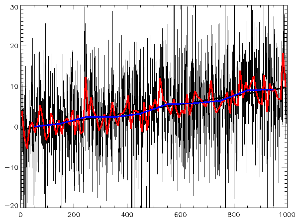
In statistics, a moving average (rolling average or running average) is a calculation to analyze data points by creating a series of averages of different subsets of the full data set. It is also called a moving mean (MM)[1] or rolling mean and is a type of finite impulse response filter. Variations include: simple, cumulative, or weighted and the exponential moving average forms.

The Moving Average Model

The moving average model in time series analysis smoothens the time series curve by computing the average of all the data points in a fixed-width sliding window and replacing those points with the computed value. The sliding window size (w) is fixed, and the window moves with a specified stride over the data, creating a new series from the average values.

Together with the autoregressive (AR) model, the moving-average model is a special case and key component of the more general ARMA and ARIMA models of time series, which have a more complicated stochastic structure. Contrary to the AR model, the finite MA model is always stationary.

The ARIMA method is similar to a linear regression equation where the prediction depends on the (p,d,q) parameters of the ARIMA model.

p: is the number of Auto-Regressive (AR) terms. For example, if p=3, the predictor for y(t) will be the terms y(t-1), y(t-2), and y(t-3).
q: is the order of the Moving Average (MA). For example, if q=3, the terms for estimating the predictor y(t) will be the terms y(t-1), y(t-2), and y(t-3).
d: is the number of differentiations to produce a stationary time series.

To determine the values of p and q, a graphic method can be used involving the following:

The Autocorrelation Function (ACF), which compares the correlation between two consecutive values but with a lag.
The Partial Autocorrelation Function (PACF), which measures the association degree between y(t) and y(t-p).

The values of p and q are integer numbers, and they can be obtained from the plots of ACF and PACF. This happens when these graphs cross the 1.96 σ line, where σ is the standard deviation. The crossing of ACF gives information about q and the PACF gives the information about p.

We will work each case: the autoregression AR and moving averages MA and then integrate them in the ARIMA model.

The Akaike Information Criterion (AIC) will be used to select the best model. The best model is the one that has the lowest AIC value.

After this, with the best ARIMA model, we will construct the Time Series Model (Tmax and Tmin).

If the time series has some seasonality component, then it is better to apply the SARIMA model.

📝 The moving-average model should not be confused with the moving average, a distinct concept despite some similarities.

ARIMA (Autoregressive Integrated Moving Average) and SARIMAX (Seasonal Autoregressive Integrated Moving Average with Exogenous Variables) are both time series models used for forecasting. They both have their own advantages and are commonly used in different scenarios.

The advantages of ARIMA models include:

Simplicity: ARIMA models are easy to understand and interpret, making them accessible to non-experts.
Flexibility: ARIMA models can be used to model a wide variety of time series data, including non-seasonal and seasonal data.
Stationarity: ARIMA models require that the time series data be stationary, which can help to improve the accuracy of the forecasts.

The advantages of SARIMAX models include:

Incorporation of exogenous variables: SARIMAX models can incorporate external variables that may affect the time series being modeled, providing a more accurate forecast.
Seasonality: SARIMAX models can handle seasonal time series data, which is common in many real-world applications.
Robustness: SARIMAX models are generally robust to outliers and missing data, making them a good choice for modeling time series data with irregularities.

In summary, ARIMA models are useful for modeling non-seasonal time series data, while SARIMAX models are better suited for seasonal time series data that can be affected by external variables.

Please see the corresponding Jupyter Notebook Example for Time Series Analysis.