-
Notifications
You must be signed in to change notification settings - Fork 1
Supervised Machine Learning: Regression Algorithms
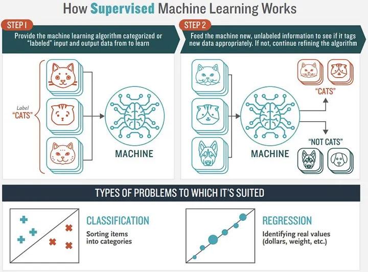
Scikit-learn is a very popular open-source machine-learning library based on Python. It supports a variety of supervised learning (regression and classification) and unsupervised learning models.

Image credits: Jorge Leonel. Medium
One list of 10 regression algorithms from Scikit-Learn, that we need to consider.
from sklearn.linear_model import LinearRegression
from sklearn.linear_model import SGDRegressor
from sklearn.preprocessing import PolynomialFeatures
from sklearn.linear_model import Ridge
from sklearn import.linear_model import Lasso
from sklearn.linear_model import ElasticNet
from sklearn.linear_model import LogisticRegression
from sklearn.svm import SVR
from sklearn.tree import DecisionTreeRegressor()
from sklearn.ensemble import RandomForestRegressor
from sklearn.neighbors import KNeighborsRegressor
Regression. Regression is predicting a continuous-valued attribute associated with an object.
Some examples of Regression algorithms included in Scikit-Learn:
- Linear Regression (Ordinary Least Squares)
-
Stochastic Gradient Descent
-
Polynomial Regression
-
Ridge Regression
-
Lasso Regression
-
Elastic Net
- Logistic Regression
- Support Vector Machines Regressor
-
Decision Tree Regressor
-
Random Forest Regressor
-
K-Nearest Neighbors Regressor

Regression metrics:
- R squared or coefficient of determination
- Mean squared error (MSE)
- Root-mean-squared error (RMSE)
- Sum of squares residuals (SSR)
- Mean absolute error (MAE)
The scikit-learn library includes a large collection of regression metrics that can be used for measuring the performance of the algorithms.
- sklearn.metrics.mean_squared_error
- sklearn.metrics.mean_absolute_error
- sklearn.metrics.r2_score
- sklearn.metrics.explained_variance_score
- sklearn.metrics.mean_pinball_loss
- sklearn.metrics.d2_pinball_score
- sklearn.metrics.d2_absolute_error_score
Please open this Notebook in Google Colab.
An example R script for performing a linear regression (ordinary least squares):
# Load the dataset
data <- read.csv("dataset.csv")

# View the first few rows of the dataset
head(data)

# Perform a linear regression
fit <- lm(dependent_variable ~ independent_variable, data=data)

# View the summary of the regression results
summary(fit)

# Calculate R-squared
rsq <- summary(fit)$r.squared

# Calculate MSE
predicted_values <- predict(fit, data)
mse <- mean((predicted_values - data$dependent_variable)^2)

# Calculate RMSE
rmse <- sqrt(mse)

# Print the metrics
cat("R-squared:", round(rsq, 3), "\n")
cat("MSE:", round(mse, 3), "\n")
cat("RMSE:", round(rmse, 3), "\n")

# Plot the regression line
plot(data$independent_variable, data$dependent_variable, main="Linear Regression", xlab="Independent Variable", ylab="Dependent Variable")
abline(fit, col="red")
An example R script for performing a polynomial regression of order n=2:
# Load the dataset
data <- read.csv("dataset.csv")

# View the first few rows of the dataset
head(data)

# Perform a polynomial regression
fit <- lm(dependent_variable ~ poly(independent_variable, 2), data=data)

# View the summary of the regression results
summary(fit)

# Plot the regression line
plot(data$independent_variable, data$dependent_variable, main="Polynomial Regression", xlab="Independent Variable", ylab="Dependent Variable")
lines(data$independent_variable, predict(fit), col="red")
- Introduction to Machine Learning with Scikit-Learn. Carpentries lesson.
- Scikit-learn cheat sheet: methods for classification & regression. Aman Anand.
- A Beginner’s Guide to Regression Analysis in Machine Learning. Aqeel Anwar. Towards Data Science, Medium.
- Learn regression algorithms using Python and scikit-learn. IBM Developer.
- 7 of the Most Used Regression Algorithms and How to Choose the Right One. Dominik Polzer. Towards Data Science, Medium.
- Regression Analysis in Machine learning. Java T Point.
Created: 02/22/2023 (C. Lizárraga); Last update: 05/02/2023 (C. Lizárraga)
University of Arizona, Data Science Institute, 2023.
- An Overview of Machine Learning Algorithms.
- An Overview of Deep Learning Algorithms
- An introduction to Machine Learning with Scikit-Learn
- Supervised Machine Learning: Classification Algorithms
- Supervised Machine Learning: Regression Algorithms
- Unsupervised Machine Learning: Clustering Algorithms
- Unsupervised Machine Learning: Dimensionality Reduction
- Introduction to Large Language Models
- Using ChatGPT in Data Science
- Use of GPT or LLM in Data Science
- Prompt Engineering Basics for Educators
- Using ChatGPT and Bard in Higher Education
- Python & General Tools for Data Science Resources
- A Data Science Digital Library
- Machine Learning Resources
Carlos Lizárraga, Data Lab, Data Science Institute, University of Arizona, 2023.
