Lucene is a Java library which provides information retrieval capabilities. Solr/Elastic Search run as stand-alone servers and provide convenient wrappers on top of Lucene's search functionality. They are both popular options for internet search engines.
The purpose of this project is to demonstrate the scoring formula which Lucene uses to calculate search relevance.
Clone repo and run python -i search_engine.py.
products = json.load( open('movies.json') )
search_engine = SearchEngine(docs=products, use_field_norms=False)
field_boosts = {'title': 1.1}
query = search_engine.query("gi joe ww2 documentary", field_boosts=field_boosts, num_results=10)
Options
- use_field_norms (boolean): Factor in field length for TD-IDF scoring
- num_results (int): Total results to display
- field_boosts (dict[string, int]): Boost certain fields by an exponent
- Search products (query -> docs)
- Similiar products on a product page (doc -> docs)
- Personalized suggestions based on user history (docs -> docs) by clustering similiar docs (example, wikipedia)
Search is a balance of precision and recall. Lucene is dumb by default; only exact words will be a match leading to great precision, but terrible recall (too many false negatives). To better search relevance, all terms go through a tokenization process (docs at index time, query at runtime). Tokenization associates different forms of a term so the recall will be greater.
Some tokenizations (see here):
- Lower case
- Strip punctuation
- Split field by white space
- Remove possessives: "Man’s" -> "Man
- Stemming: "Jumping" -> "Jump"
- Phonetic: BMPM: "In its current implementation, BMPM' is primarily concerned with matching surnames of Ashkenazic Jews..." website
- N-Gram: Each combination of n chars for a term. "hello" for 2-3 chars is ["he", "el", "ll", "lo", "hel", "ell", "llo"]
- Edge-N-Gram: Each combination of n chars for a term from start of word. "hello" for 3+ chars is ["hel", "hell", "hello"]. Very useful for autosuggest while user typing.
- Bigrams: Pairs of words
| Term | Explanation |
|---|---|
| Doc | Record from CSV/JSON/HTML/PDF/DB, etc. |
| Term | Subset of field, could be letter, word, or any n-chars. |
| Weight | Value of term within a field of doc |
| TF | Term Frequency within a field |
| IDF | Rarity of term within doc (Inverse Doc Frequency) 1/DF |
| fieldNorm | Shorter fields have more weight than longer ones |
| field_boost | Boost a term match if found in field x by an exponent of n |
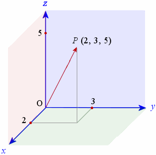
The vector model views both the query and the searchable documents as a vector on a mullti-dimensional graph.
Each axis of the graph represents a term and the value on the axis is the weight of the term within the doc or query.
The vectors will only have numbers >= 0. Doc vectors with axis's of 0 indicate that a particular term has no match in the query vector and can be safely ignored.
There are two components to understand:
- How we procure the value of a particiular axis (the weight of a term). These calculations are done at index time.
- How we calculate the similiarity between two vecors (query <-> docs) .
The weight of a matching term is scored by the frequency of the term within the given field (TF) multiplied by how rare the term is within the set of documents (IDF).
Practically, the a variation of the this formula is generally used:
| Name | Formula | Query | Document |
|---|---|---|---|
| IDF | log( doc_count / num_docs_which_contain_term ) + 1 ) + 1 | YES | YES |
| TF | sqrt(field.count(term)) | NO | YES |
| fieldNorm | 1 / sqrt( num_chars_in_field) | NO | YES |
| field_boost | query['term_in_boosted_field']**field_boost | YES | NO |
For a query, TF is irrelevant since query rarely contain duplicate words. fieldNorm is also not important; queries are usually concise.
Here is an example for a query of gi joe ww2 documentary.
fieldNorms are set to True and field_boosts are {'title': 1.1, 'genre': 1.5}:
# query vector
{'documentary': {'score': 5.015173140485178},
 'gi': {'score': 8.965719169172438},
 'joe': {'score': 5.642844374217615},
 'ww2': {'score': 0}}

# top result vector for doc 11838
{'gi': {'field_name': 'title',
        'field_text': 'The Story of G.I. Joe',
        'score': 1.956480321545204},
 'joe': {'field_name': 'title',
         'field_text': 'The Story of G.I. Joe',
         'score': 1.2313695942718068}}

# original record
{'cast': ['Burgess Meredith', 'Robert Mitchum'],
 'genres': ['War'],
 'title': 'The Story of G.I. Joe',
 'year': 1945}

# doc weights from index
{'cast': {'burgess': 1.2106351225005683,
          'meredith': 1.1461898093155403,
          'mitchum': 1.1096031454459072,
          'robert': 0.6646962483369104},
'genres': {'war': 1.8221135281634746},
'title': {'gi': 1.956480321545204,
           'joe': 1.2313695942718068,
           'of': 0.7117316180615629,
           'story': 1.3784931651895422,
           'the': 0.5162296287278824},
'year': {'1945': 2.625807684692801}}Since everything is a vector we can use known formulas from geometry to compare them.
Step 1 - calculate dot product.
Note that since 'gi' and 'joe' were found in a boosted field ('title'), we apply the exponent (1.1).
query['documentary'] * doc['documentary'] +
query['gi']**field_boost['title'] * doc['gi'] +
query['joe']**field_boost['title'] * doc['joe'] +
query['ww2'] * doc['ww2'] +
= dot_product

5.015173140485178 * 0 +
8.965719169172438^1.1 * 1.956480321545204 +
5.642844374217615^1.1 * 1.2313695942718068 +
0 * 0 = 30.1044142369

dot_product = 30.1044142369
Step 2 - incorporate coord (coordination factor) punish score for missing query terms
dot_product = dot_product * ( matching_terms / num_terms_in_query )
dot_product = 30.1044142369 * (2/4) = 15.0522071184
Step 3 - cosine similarity (rebalance to 0-1 decimal)
def norm(vector):
	return sqrt(sum(value['score']**2 for value in vector.values()))

dot_product / norm( query_vector ) * norm( doc_vector )

15.0522071184 / ( 11.720826527218524 * 2.3117279957405756)
cosine_similarity = 0.55552705533
This is how the code prints out the top result:
------------------------------------------------
Ranking Score   Idx   Terms
1       0.5555  11838 joe, gi
title - The Story of G.I. Joe
------------------------------------------------
