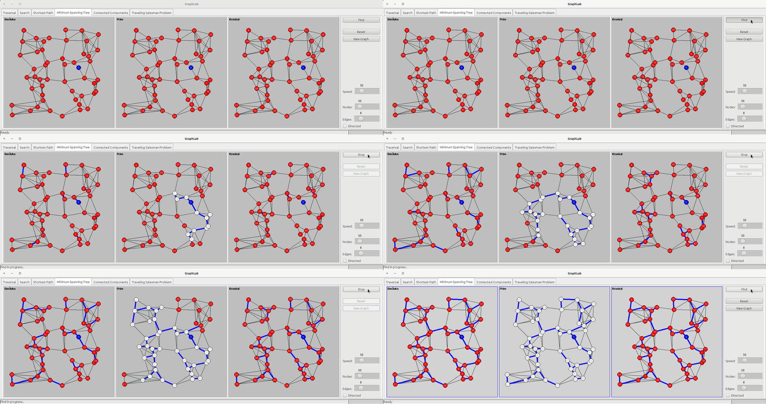
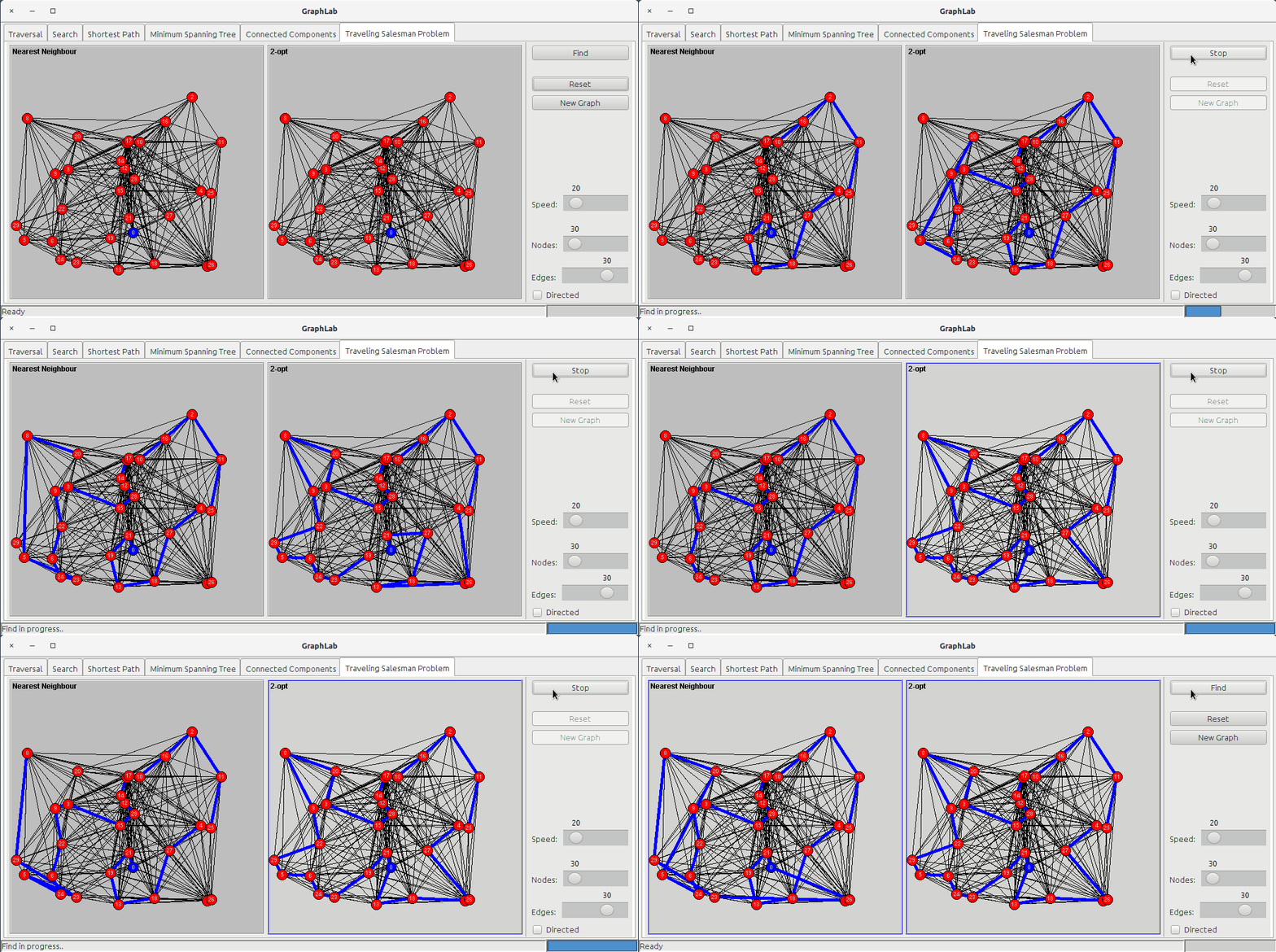
is a Java Swing application that shows visually how works several graph algorithms. The application has several tabs, each of them showing a particular algorithm; each tab has a control panel on the right that let the user start the execution, stop it and create new graphs using sliders for deciding how many random nodes/edges to create and if directed or not. The user can also set a specific node as the starting node or move the nodes along the canvas just by dragging and dropping them on another position.
The application has now six tabs:
- Traversal
- Search
- Shortest Path
- Minimum Spanning Tree
- Connected Components
- Traveling Salesman Problem
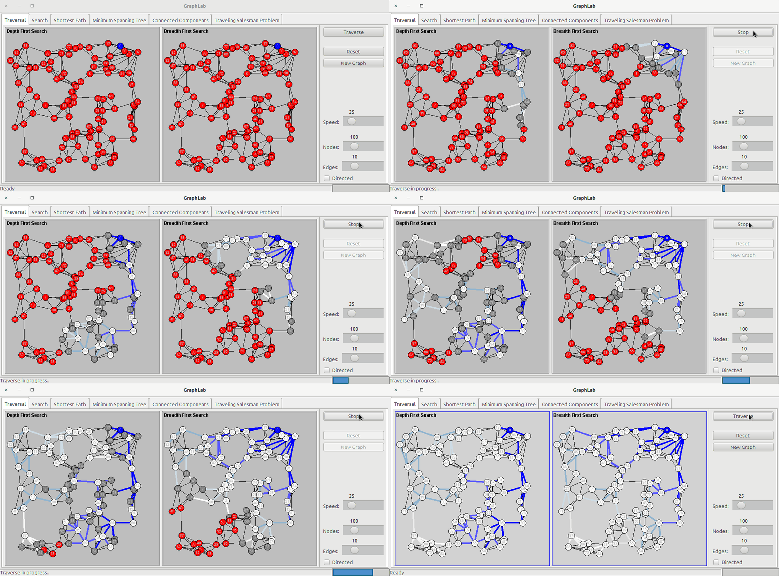 The traversal tab shows two panels:
- DFS (Depth First Search)
- BFS (Breadth First Search)
Before starting the traversal every node is red (UNKNOWN) and the edges are thin; while it executes the algorithms, it changes the color of a node to grey (DISCOVERED) and then to to white (PROCESSED) and also the color of the edges, which start blue and then shade to white as long as they get further from the starting node. The difference between DFS and BFS will be highlighted by the visualization since in BFS all the edges around the starting edge will be blue or light blue, and becoming white in circular patterns; in DFS, on the other hand, the color of the edges will follow the neighbors of every node, and the path can be very convoluted.
DFS is a graph traversal algorithm that consists of these steps:
- select a starting node as current node
- for each neighbors of this node
- select this neighbor as current node
- goto step 2
This means that the algorithm will traverse in depth all the edges of the graph, since it will begin with the starting node, then it will choose its first neighbor, then it will choose its first neighbor, ..., and so on.
DFS has lower memory consumption compared to BFS.
BFS is a graph traversal algorithm that consists of these steps:
- select a starting node as current node
- for each neighbors of this node
- put this neighbor in a queue
- select first element from queue as current node
- goto step 2.
This means that the algorithm will traverse in breadth all the edges of the graph, since it will begin with the starting node, then it will put all its neighbors in a queue, then it will get the first neighbor of the starting node and it will put all its neighbors in the queue, then it will get the second neighbor of the starting node and it will put all its neighbors in the queue, ..., and so on.
BFS has higher memory consumption compared to DFS and is suitable when searching for a shortest path from the starting node to any node in the graph.
For more detailed info on these algorithms check Wikipedia for DFS and BFS.
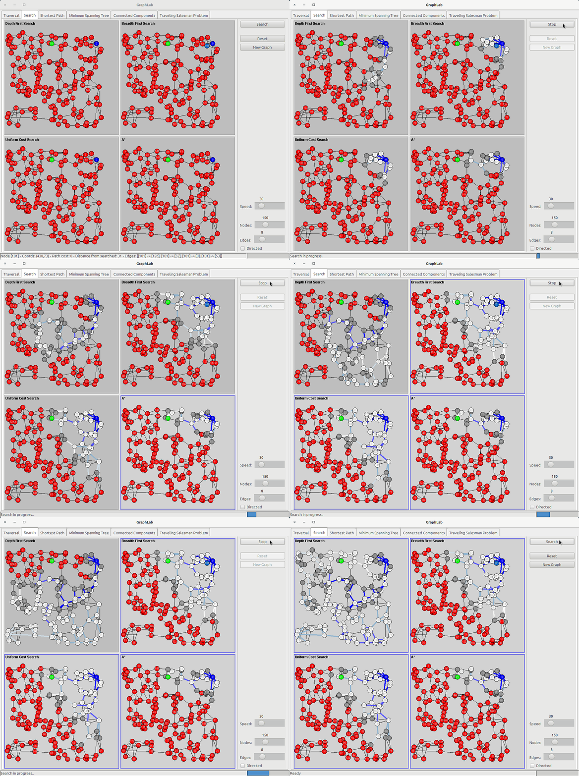 The search tab shows four panels:
- DFS (Depth First Search)
- BFS (Breadth First Search)
- UCS (Uniform Cost Search)
- A* (A star)
Instead of just traversing the graph, for searching we start from a node and we want to reach a destination node (usually called goal).
see above description
see above description
The Uniform Cost Search is based on the idea of BFS, but instead of putting nodes into a queue, it uses a Priority Queue where the value to prioritize is the edge cost (or, better, the sum of all the costs of the edges from the starting node); so UCS is a Greedy Algorithm where the cheapest edges are chosen first.
The A star algorithm adds the concept of heuristic function, which is a function that takes a node as argument and returns a value that tells how good is that node for our goal (the lower the value, the better is). If the heuristic function satisfies two rules:
- it never overestimates the value for the node
- the triangle inequality holds
then the algorithm is guaranteed to be optimal. In GraphLab application, the heuristic function is the euclidean distance between a node and the goal node, so that the nodes that are closer to our goal are visited first.
Check Wikipedia for more details: A* search
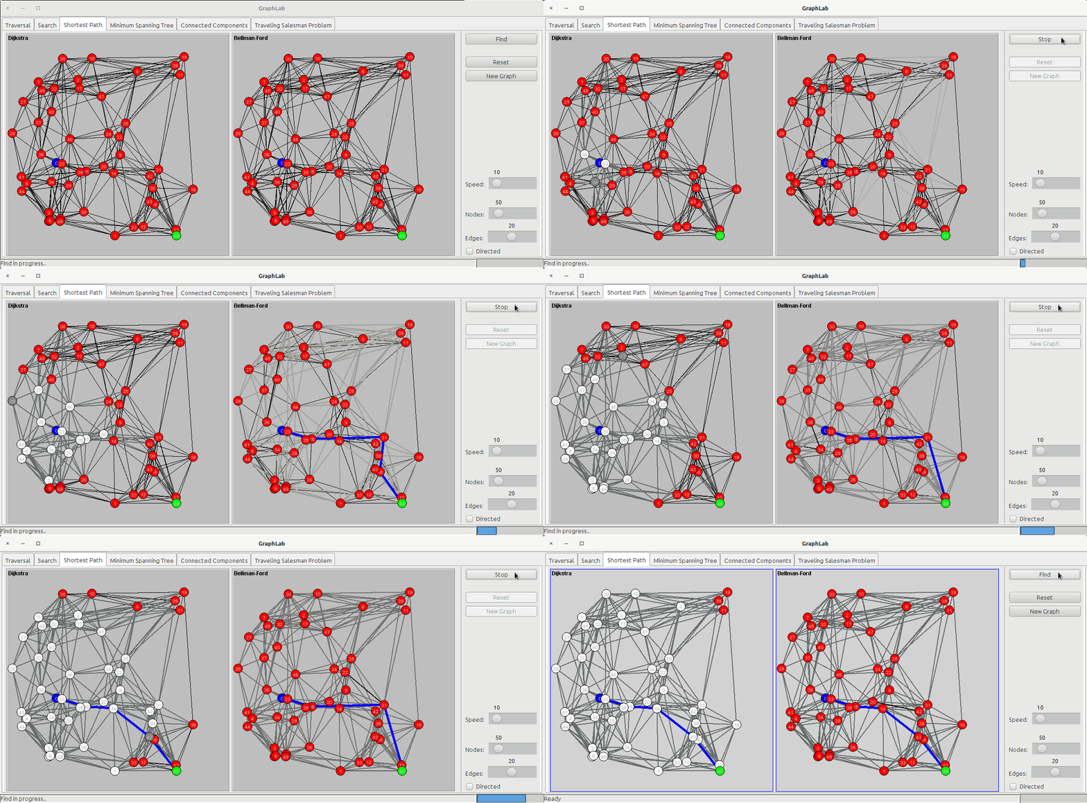 The shortest path tab shows two panels:
- Dijkstra
- Bellman-Ford
As in the search tab, for the shortest path we start from a node and we want to find the shortest way to arrive to a destination node (usually called goal).
The Dijkstra's algorithm uses a Priority Queue to store all the nodes to visit based on the cost of arriving to that node passing from the cheaper edges. It works by visiting all the nodes and incrementing the total cost fo the node with the cost of the last edge. In my implementation, once the algorithm has processed the goal node, it stops, while other implementations let the algorithm run on all the nodes of the graph.
If edge costs are negative, this algorithm will not work.
The Bellman-Ford algorithm doesn't care about nodes, but only edges: it loops over the edges V-1 times to obtain the shortest path: at the end of the search, the nodes will be colored in red (the UNKNOWN status) because they have not been visited. This algorithm can be used also when edge costs can be negative.
The minimum spanning tree is a subset of the edges of a connected, edge-weighted undirected graph that connects all the vertices together, without any cycles and with the minimum possible total edge weight.
The minimum spanning tree tab shows three panels:
- Borůvka
- Prim
- Kruskal
Borůvka's algorithm starts examining each node and adding the cheapest edge of that node without regard to already added edges, and keeps joining these groupings in a like manner until a tree spanning all vertices is completed.
Prim's algorithm starts from a node and then keeps adding new nodes to the tree, choosing the cheapest possible connection to the tree at every step.
Kruskal's algorithm only consider edges; it starts sorting the edges based on their cost and then keeps grouping edges together (following the ascending cost order) until they are all connected, forming a tree.
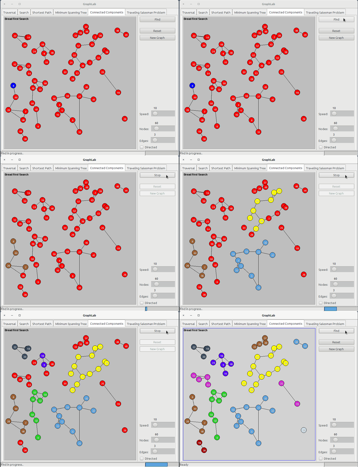 The connected components tab shows one panel:
- BFS
A BFS traversal is used to visit all the edges of the graph and at the end of execution is made a check on the number of visited nodes: if it's lower then the number of nodes of the graph, it means that there are other nodes not touched by the preceding traversal. The algorithm will then loop over all the nodes of the graph looking for the first that has not been visited for starting a BFS on that node too. The operation is repeated until there are no more unvisited nodes. Every component of the graph is shown in a different color.
The traveling salesman problem is a famous NP-Complete problem (check wikipedia page. The traveling salesman problem tab shows two panels:
- Nearest Neighbor
- 2-opt
The nearest neighbor is a Greedy Algorithm that begins on the starting city and then tries the cheapest edge to unvisited cities and repeat this process until it finds a tour (usually not optimal) using backtracking.
The 2-opt algorithm starts from a valid tour (not optimal) and tries to optimize it checking every couple of edges and seeing if swapping them lowers the total cost; if true, it sets the updated tour as the starting tour and repeat the process until it find no swaps that lower the total cost. In this implementation, the first tour is obtained by the nearest neighbor.
- Java 8 (with the java executable available in path)
The project is built with Maven, so to create the JAR you just need to launch:
mvn clean install
and then launch it with:
java -jar target/GraphLab.jar
