Plugging TensorBoard in an autoencoder on the MNIST dataset for demonstrating t-SNE embeddings visualization of unsupervised machine learning.
Note that what t-SNE gives us are embeddings too. To be clear, in this project, we have two types of embeddings:
- We embed and compress the dataset with an autoencoder. This is an unsupervised neural compression of our data and such neural compressions can reveal to be very useful for various tasks where unlabeled data is available.
- We embed the autoencoder's embedding with t-SNE as a mean to further compress the information to visualize what's going on in the autoencoder's embeddings. This is really a visualization of what's going on.
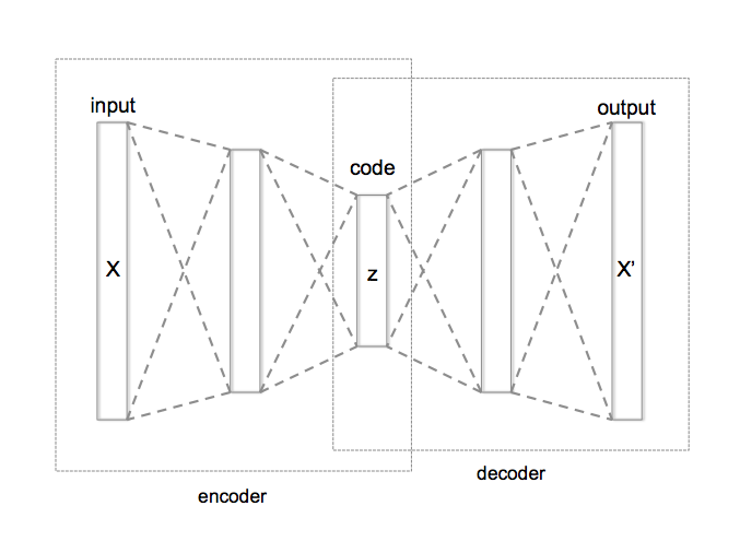
The nuance here compared to running t-SNE embeddings on the raw mnist input images is that we visualize what the encoder has managed to encode in its compressed, inner layer representation (called "code" in the picture below, and often called "embedding").

The encoder we train here is very simple just to give an example with a code of 64 neurons wide. Ideally, it would contain convolutions and would be more optimized.
You may want to read this great article on how to interpret the results of t-SNE. Here is how does t-SNE looks like with the default parameters (perplexity of 25 and learning rate of 10):
Note that a Principal Component Analysis (PCA) can be used in a similar way. However, a PCA is a bit more interesting mathematically than t-SNE, despite t-SNE looks better to the human eye. Here is how a PCA looks like, representing 19.8% of the variance:
Run:
python3 autoencoder_t-sne.py
./run_tensorboard.sh
You could also simply run the same thing that's contained in the .sh:
tensorboard --logdir=logs --port="6006"
That simply runs TensorBoard on its default port.
Browse to localhost:6006 or http://0.0.0.0:6006/ and then head to the "embedding" tab.
Choose to color by label and then you may play with t-SNE or PCA embeddings!
Enjoy!

