Follow the below links download and install the appropriate version of R and R Studio for your operating system
Download the workshop files by clicking the green "clone or download" button and then click "Download ZIP". Move the resulting folder to your desktop.
Download the data we will use in the workshop from the below link. The resulting file should be a compressed "2008.csv.bz2" file. Uncompress the file and move the file into the R_Workshop folder on your desktop. Once it is uncompressed you should have a 689.4mb file named "2008.csv" in R_Workshop folder.
or
download.file(url="https://s3.amazonaws.com/stat.184.data/Flights/2008.csv",destfile='2008.csv', method='curl')
download.file(url="https://s3.amazonaws.com/stat.184.data/Flights/airports.csv",destfile='airports.csv', method='curl')
R has a "working drectory" which is the folder where R will load data from and write files out to; You will need to set the working directory in the R GUI, the R-Studio GUI or by writing in the command line:
setwd("~/Desktop/R_Workshop")
The utility of R is in the hundereds of packages which offer thousands of pre-made functions. Packages will need to be installed; you can install them in the R GUI, the R-Studio GUI or by writing in the command line:
install.packages("data.table")
Once packages are installed you will still need to load them in order to use their functions; you can load them with the 'library()' function:
library(data.table)
This workshop will leverage functions from several packages, you can install and load all of them with the following command:
source("Workshop_Packages.R")
R has some basic data structures we will primarily use just two, vectors and data_tables
Vec <- 7 #this is a vector
num_Vec <- c(1,2.5,3,4.7) #this is also a vector
Log_Vec <- c(TRUE,TRUE,FALSE,TRUE) #this is a vector of logical statements
Chr_Vec <- c("This", "is a", "character", "vector") #this is a character vector
DT1 <- data.table(V1=num_Vec,V2=Log_Vec,V3=Chr_Vec) #DT1 is now a data.table
str(DT1) #the str() function will tell you about the types of each column in a data.table
Indexing allows you to retrieve values or subset a data_table
DT1[1,] #returns the first row, notice that this is a data_table
DT1[,V2] #returns the column named "V2", notice that this is a vector
".csv" files are a common way to store data, we can load ".csv" files with the fread() function:
DT<-fread("2008.csv") #This reads in the flight data and stores it as an object called 'DT'
AP<-fread("airports.csv") #This reads in the data about airports and stores it as an object called 'AP'
We can now look at the data with some useful functions
dim(DT) #the dim() function will show you the number of rows and the number of columns in a data_table
DT #this is okay with a data_table but it is bad practice
head(DT) #this is the preferred way to look at the top of an object
tail(DT) #this is the preferred way to look at the bottom of an object
str(DT) #we learned about data types above, this is a useful way to inspect a data object and see column types
Data Wrangling is the process of subsetting, reshaping, transforming and merging data. Lets begin by merging the two data tables together. We'd like to merge using the Airport codes (a common value between datasets), but they are named "iata_code" in the Airports dataset and "Origin" and "Dest" in the Flights dataset. We will be focusing on departure delays in our analysis so we will be merging to "Origin".
setnames(AP,"iata_code","Origin") #this changes the name of the "iata_code" column to "Origin"
setkey(DT,Origin) #before merging we can re-order the datasets by what we want to merge on
setkey(AP,Origin) #this will match the order for both data frames, this will significantly speed up the merge
DT<-merge(DT,AP,all.x=T) #Now we can merge, notice the "all.x=T"
Now we will subset the large dataset to just the Washington DC area airports.
WashAP<-c('DCA','IAD','BWI') #we can make a vector
WF<-DT[Origin %in% WashAP] #then using that vector to subset
dim(WF)
WF<-WF[Cancelled==0] #we can also use a logical statement
Sometimes we will want to re-organise or summarize data, the dcast() function is useful for that
Avg_tab<-dcast(WF,Origin ~ UniqueCarrier,mean,value.var= c("DepDelay"))
Avg_tab #this is a useful way of looking at summary stats but notice that it is not 'tidy'
Based on that view we can see that there are a number of carriers in the data set, many of them do not operate out of all three Washington area airports. Lets limit our analysis to just the four major passanger airlines.
MPasAl<-c('AA','DL','UA','US') #making a vector
WFsub<-WF[UniqueCarrier %in% MPasAl] #subsetting with a vector
Character or "string" vectors are a common data format, the 'stringr' package is desighned to help with string manipulation
WFsub$Month<-str_pad(WFsub$Month,2,side="left",pad="0") #we will use the str_pad() function to format our date columns
WFsub$DayofMonth<-str_pad(WFsub$DayofMonth,2,side="left",pad="0")
WFsub$CRSDepTime<-str_pad(WFsub$CRSDepTime,4,side="left",pad="0")
WFsub$DepDateTime <-paste0(WFsub$Month,WFsub$DayofMonth,WFsub$Year," ",WFsub$CRSDepTime) #the paste0() function will concatenate columns
data assosiated with dates can be particularly tricky to deal with, the lubridate package is desighned to help with date related data formating and transformation
WFsub$DepDateTime <-parse_date_time(WFsub$DepDateTime,"%m%d%Y %H%M") #make a new column with both the date and the time
WFsub$TimeOnly <-parse_date_time(WFsub$CRSDepTime,"%H%M") #make a new column with just the time
ggplot2 is the prefered package for data visualization in R
It is often best to start with a relativly simple plot and work toward a more complicated but clearer plot iterativly
ggplot(WFsub,aes(x=TimeOnly,y=DepDelay,col=UniqueCarrier))+geom_point()+scale_x_datetime(date_breaks= "2 hours",date_labels ="%r")
We can remove the points and replace with a smooth plot and break the plot into facets by airport:
ggplot(WFsub,aes(x=TimeOnly,y=DepDelay,col=UniqueCarrier))+facet_wrap(~name,ncol= 1,scales = "free_x")+geom_smooth()+coord_cartesian(ylim=c(0,30))+theme_minimal()+scale_x_datetime(date_breaks= "2 hours",date_labels ="%r")
The ggsave function will save the plot as a ".pdf"
ggsave("WashAreaAirport_Delay_by_Hour.pdf")
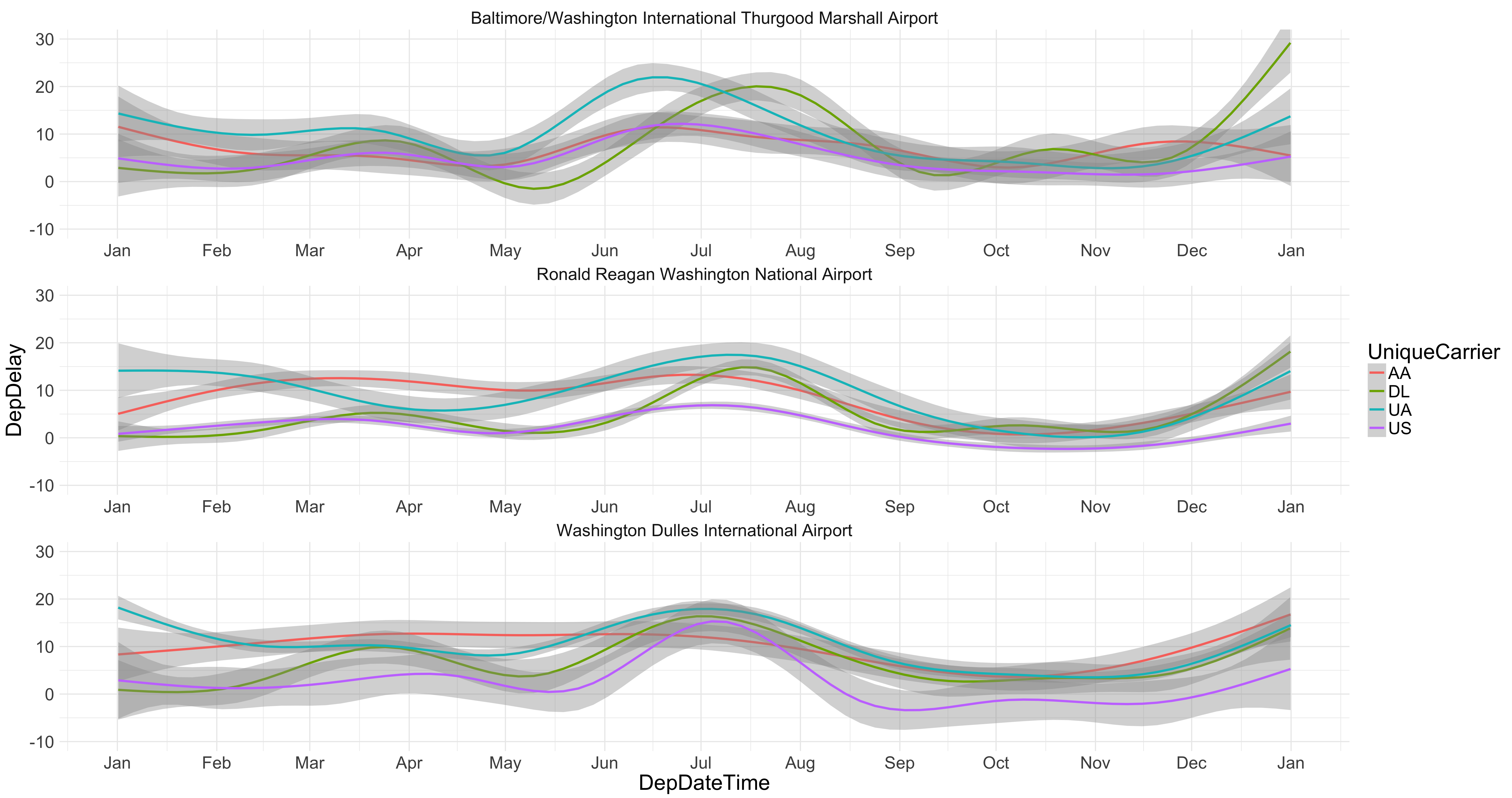
We can also look at the trends across the year
ggplot(WFsub,aes(x=DepDateTime,y=DepDelay,col=UniqueCarrier))+facet_wrap(~name,ncol= 1,scales = "free_x")+geom_smooth()+coord_cartesian(ylim=c(-10,30))+theme_minimal()+scale_x_datetime(date_breaks= "1 month",date_labels ="%b")
ggsave("WashAreaAirport_Delay_by_Month.pdf")

