-
Notifications
You must be signed in to change notification settings - Fork 12
Stats
PyForecast uses a variety of modern statistical concepts to generate relevant and powerful statistical models. The following section describes the major statistical concepts in detail.
The general principle in developing a seasonal, statistically-based streamflow volume forecast is to use a multiple linear regression model relating current climatic information, such as snowpack, accumulated precipitation and streamflow, air temperature, and climatic indices to future accumulated streamflow at a given point, for a specified period of time. In the Western United States, accumulated snowpack in the winter and spring can be highly correlated to snowmelt runoff.
For example, a multiple linear regression model may relate April 1 snowpack measurements, March 1 through March 31 accumulated streamflow, and April 1 El Nino Southern Oscillation Indices to April 1 through July 31 streamflow at a given point. A forecast for future April through July streamflow is created on April 1 by using the current measurements for these variables in the multiple linear regression model to develop a median forecast. The uncertainty distribution associated with the multiple linear regression model typically describes the forecast uncertainty.
PyForecast builds upon the techniques described in (Garen, 1992). Garen described four key improvements to statistical forecasting at the time:
- Basing the regression model only on data known at forecast time (no future data);
- principal components regression;
- Cross-validation; and
- systematic searching for optimal or near-optimal combinations of variables.
These areas are described in further detail below.
More recent improvements to statistical seasonal forecasting are described in (Perkins, Pagano, and Garen, 2009). This included the use of z-score regression.
According to (Rencher and Schaalje, 2008), a linear regression model describes the relationship between a dependent or response variable and an independent or predictor variable. Key assumptions of linear regression are that the model is linear, and certain assumptions about error distributions.
When a response variable is influenced by multiple predictor variables, multiple linear regression is used. Multiple linear regression relates several predictor variables to a single response variables, again with the assumptions of error distributions and linearity.
Streamflow forecasters typically utilize multiple linear regression models to predict future events. Extensive datasets exist describing the conditions within the non-homogenous watersheds we forecast, limiting the usefulness of simple linear regression. PyForecast's application of multiple linear regression is described below.
If the user is generating forecast equations using the Multiple Linear Regression section of the Regression Tab, then the program evaulates each model iteration using a standard least-squares regression of predictors against the predictand. The procedure, which incorporates cross-validation, is detailed below.
The program starts with an array of predictor and predictand data, for example:

The program then splits the data according to the user's chosen cross-validation method. Actual model fitting is performed using the Numpy Linear Algebra library. The coefficients and intercept that are ultimately stored in the model are generated using the full set of data, not one of the split datasets.
According to (Helsel and Hirsch, 2002):
Principal components are linear combinations of the p original variables which form a new set of variables or axes. These new axes are uncorrelated with one another, and have the property that the first principal component is the axis that explains more of the variance of the data than any other axis. The second principal component explains more of the remaining variance than any other axis which is uncorrelated with (orthogonal to) the first. The resulting p axes are thus Graphical Data Analysis new "variables", the first few of which often explain the major patterns of the data in multivariate space. The remaining principal components may be treated as residuals, measuring the "lack of fit" of observations along the first few axes.
PyForecast uses principal components to create orthogonal variables from the highly correlated predictor variables available for forecasting, such as snow water equivalent measurements throughout a basin or streamflow measurements on tributary streams. The orthogonal variables are then used to create a multiple linear regression model for predicting future streamflow volumes. PyForecast's application of principal components is described below.
When a user elects to generate a principal components forecast, the program evaluates each model iteration by doing the following:
- Decomposing the predictor data into Principal Components
- Determines which set of Principal Components [(PC1), (PC1,PC2), ..., (PC1, PC2, PC3, ..., PCN)] generates the most skillfull MLR model (with cross validation)
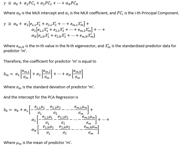
- Recomputes the original, non-transformed model coefficients and intercept
The program computes the coefficient and intercept as follows:
Z-score regression creates composite predictor variables for multiple linear regression by scaling individual predictors by the mean and standard deviation, and weighting the individuals by the coefficient of determination (r-squared). This method allows for the use of stations with missing data within the historical record. PyForecast's implementation of Z-score regression appears below.
When a user elects to generate a Z-score Regression, the program evaluates each model iteration by doing the following (Largely follows the z-Score technique in the VIPER Technical Note).
- Constructing the composite dataset from standardized predictor data
- Using Linear Regression to regress the composite dataset against the predictand.
- Returning the original, un-transformed coefficients and intercept.
The statistical technique varies slightly from the VIPER procedure. PyForecast does not compute a composite index for each data type. Instead it computes one composite index using all the data, regardless of datatypes.
When a large set of predictors exist to predict a target, it is almost always the case that a subset of the predictors will generate a more skillful model than the complete set of predictors. It is therefore in the interest of the forecaster to try a variety of predictor combinations in order to find the best regression model possible. In data science, the process of determining which variables among a set of predictors create the most skillful model is referred to as feature selection.
PyForecast uses a methodology called Parallelized Sequential Floating Selection to create well-performing regression models. The algorithm that PyForecast uses largely follows the algorithm laid out in the last two slides of this presentation. The specific steps that PyForecast uses to choose predictors are laid out below:
For sake of example, we'll assume that the forecaster is trying to develop an April 1st forecast equation from the following pool of 6 predictors:
- X1: SNOTEL STATION 1, March 31st SWE
- X2: SNOTEL STATION 1, March 15th SWE
- X3: SNOTEL STATION 2, March 31st SWE
- X4: SNOTEL STATION 2, March 15th SWE
- X5: HUC 10030101 Accumulated Precipitaion, October 01 - March 31
- X6: Reservoir Inflow, November Average
Additionally, the user has elected to generate 6 models, by setting the 'Number of Models' parameter to 6.
The program will create 6 identical models, each empty without any predictors in them:
To begin, the program will attempt to add a predictor to the first model. It looks at the predictors that are currently in the model (in this case, there are not any predictors in the model yet), and it generates a list of predictors that can still be added to the model (in this case, it can potentially add any of the 6 predictors into the model). It adds each potential predictor individually, and evaluates the resulting model. In this case, adding predictor X3 maximized the skill of the model (The skill is evaluated as the Adjusted R2, though the user could have selected RMSE or Nash-Sutcliffe it they wished). The X3 predictor is added to the model.
Next, the program will attempt to remove a predictor from the first model. It looks at the predictors currently in the model (in this case, X3 is the only predictor in the model), and generates a list of predictors that it can potentially remove. One by one, it will remove individual predictors from the model and evaluate the resulting skill. It will not attempt to remove a predictor that was just added in the previous step (this would return the model to its original state, getting us nowhere). If removing a predictor from the model increases the skill, it will remove that predictor and continue. In this case, it will not attempt to remove the X3 predictor.
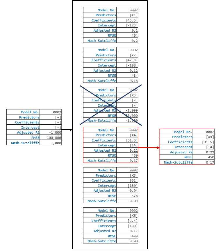
Now, the program will move on to the second model, and attempt to add a predictor to that model. It will generate a list of potential predictors to add, add each on individually, and assess the skill of each addition. The program will also check to make sure that the predictor addition does not result in a model that already exists. In this case, if the program were to add X3 to the model, then model 0002 could potentially be the same as model 0001. Therefore, it will not even consider adding X3 to the model, and will disregard it entirely. In our case, because it could not add X3, the next best predictor to add was X4. X4 is added to the second model.
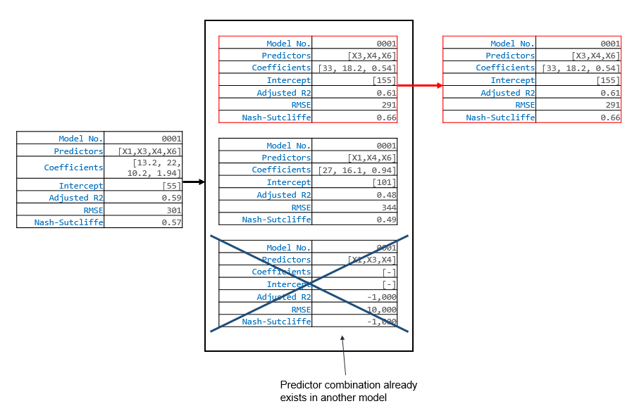
The program will continue in this manner until it can start removing predictors (that is when models start containing 2 or more predictors). For example, in the next iteration, the program might decide to add X1 to model 0001, so that model 0001 now contains the predictors X1 and X3. After it adds X1, it can now evaulate the effects of removing X3. In this case, we know that removing X3 will result in a less skillfull model because we already analyzed that possibility above. But if we were a bit further along, and the program had just added X4 to model 0001 so that now the model contained X1, X3, X4, and X6, then the predictor removals become non-trivial. In that situation, the following might happen:
The program will continue to step through model additions and removals. In each iteration, a predictor is added and/or removed from each model. Sometimes the program will not add a predictor, and will just remove one. Other times it will add a predictor, and determine that it cannot remove a predictor. Eventually, the program will terminate when neither adding or removing predictors from any of the models increases the skill of that model.
The brute force method for finding well performing models simply takes all the possible combinations of predictors, evaluates each one, and keeps the best performing models based on the user-defined performance metric. As an example, a predictor set comprised of datasets A and B would yield 3 possible combinations comprised of A, B, and AB. The number of possible predictor combinations is a combinatorics problem which can be simplified with the equation X=2n-1 where n is the number of predictors and X is the number of unique combinations of predictors.
Due to the exponential growth of the number of possible predictor combinations, this method is not recommended for finding acceptable models given a large amount of possible predictors. As an example, a brute force run using 5, 10, and 20 predictors would result in 31, 1023, and 1048575 possible combinations of predictors respectively and each one of these combinations will be evaluated by the brute force method if selected. Although the software will take some time to evaluate all the models, it will only keep a running record of the best performing models based on the number of models the user specifies before running the selected regression algorithm.
For example, if the user chose K-Fold (5 splits), the program would generate and evaluate 5 datasets:
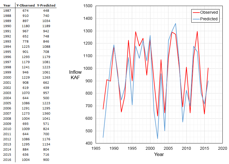
For each split of the dataset, the program will train a multiple regression model on the 'Training Data', and generate 6 predictions using the 'Testing Data' as model inputs. Then the program will stack the 30 predictions from the 5 datasets, and compute cross-validated statistics (Adjusted R2, RMSE, and Nash-Sutcliffe) between the actual observed inflows and the predicted inflows.
No data transformations are currently used or available within PyForecast. According to (Pagano et al., 2009), transformations may be useful for "nonlinear relation between predictor and predictand or in the case of heteroscedasticity in the error distribution." Data transformations are anticipated in future iterations of the PyForecast software.
The r-squared value, or coefficient of determination, is defined by the regression sum of squares divided by the total sum of squares. R-squared therefore indicates the proportion of variation in the response variable described by the model (Rencher and Schaalje, 2008). Because R-squared increases with the number of predictors in the model without increasing skill, adjusted R-squared corrects for the number of predictors in the model.
Nash-Sutcliffe Efficiency (Nash and Sutcliffe, 1970) is similar to the coefficient of determination in that it is calculated as the modeled sum of squares divided by the total sum of squares. However, because the modeled sum of squares can be greater than the total sum of squares, Nash-Sutcliffe Efficiency can be below zero. a Nash-Sutcliffe value of zero indicates the model skill is equal to predictions using the mean; values below indicate less skill and values above indicate greater skill than the mean.
RMSE measures departures from actual values and is calculated as the square root of the sum of squared error divided by the number of observations Helsel and Hirsch, 2002.. Smaller values describe predictions closer to the true value and are considered better. As with r-squared and Nash-Sutcliffe Efficiency, RMSE punishes models with larger departures (i.e., outliers) due to squaring of error. This is important when minimizing large errors is more important than minimizing average error.


