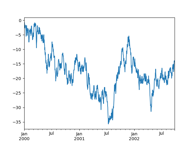
pandas is a software library written for the Python programming language for data manipulation and analysis.
import numpy as np

import pandas as pd
- Creating a Series by passing a list of values, letting pandas create a default integer index:
s = pd.Series([1, 3, 5, np.nan, 6, 8])

s
Out[4]:
0    1.0
1    3.0
2    5.0
3    NaN
4    6.0
5    8.0
dtype: float64
- Creating a DataFrame by passing a NumPy array, with a datetime index and labeled columns:
dates = pd.date_range("20130101", periods=6)
- Creating a DataFrame by passing a dict of objects that can be converted to series-like.
df2 = pd.DataFrame(
    {
        "A": 1.0,
        "B": pd.Timestamp("20130102"),
        "C": pd.Series(1, index=list(range(4)), dtype="float32"),
        "D": np.array([3] * 4, dtype="int32"),
        "E": pd.Categorical(["test", "train", "test", "train"]),
        "F": "foo",
    }
)
following show how to view the top and bottom rows of the frame:
df.head()
Out[13]:
                   A         B         C         D
2013-01-01  0.469112 -0.282863 -1.509059 -1.135632
2013-01-02  1.212112 -0.173215  0.119209 -1.044236
2013-01-03 -0.861849 -2.104569 -0.494929  1.071804
2013-01-04  0.721555 -0.706771 -1.039575  0.271860
2013-01-05 -0.424972  0.567020  0.276232 -1.087401
DataFrame.to_numpy() NumPy arrays have one dtype for the entire array, while pandas DataFrames have one dtype per column.
DataFrame.to_numpy() does not include the index or column labels in the output.
following afew dataFrame:
- describe() shows a quick statistic summary of your data:
df.describe()
Out[19]:
              A         B         C         D
count  6.000000  6.000000  6.000000  6.000000
mean   0.073711 -0.431125 -0.687758 -0.233103
std    0.843157  0.922818  0.779887  0.973118
- Transposing your data:
df.T
Out[20]:
   2013-01-01  2013-01-02  2013-01-03  2013-01-04  2013-01-05  2013-01-06
A    0.469112    1.212112   -0.861849    0.721555   -0.424972   -0.673690
B   -0.282863   -0.173215   -2.104569   -0.706771    0.567020    0.
- Sorting by an axis:
df.sort_index(axis=1, ascending=False)
Out[21]:
                   D         C         B         A
2013-01-01 -1.135632 -1.509059 -0.282863  0.469112
2013-01-02 -1.044236  0.119209 -0.173215  1.212112
2013-01-03  1.071804 -0.494929 -2.104569 -0.861849
- Sorting by values:
df.sort_values(by="B")
Out[22]:
                   A         B         C         D
2013-01-03 -0.861849 -2.104569 -0.494929  1.071804
2013-01-04  0.721555 -0.706771 -1.039575  0.271860
2013-01-01  0.469112 -0.282863 -1.509059 -1.135632
- Selecting a single column, which yields a Series, equivalent to df.A:
df["A"]
Out[23]:
2013-01-01    0.469112
2013-01-02    1.212112
2013-01-03   -0.861849
2013-01-04    0.721555
- Selecting via [], which slices the rows.
df[0:3]
Out[24]:
                   A         B         C         D
2013-01-01  0.469112 -0.282863 -1.509059 -1.135632
2013-01-02  1.212112 -0.173215  0.119209 -1.044236
2013-01-03 -0.861849 -2.104569 -0.494929  1.071804
- For getting a cross section using a label:
df.loc[dates[0]]
- Selecting on a multi-axis by label:
df.loc[:, ["A", "B"]]
- Showing label slicing, both endpoints are included:
df.loc["20130102":"20130104", ["A", "B"]]
- Reduction in the dimensions of the returned object:
df.loc["20130102", ["A", "B"]]
- For getting a scalar value:
df.loc[dates[0], "A"]
- Select via the position of the passed integers:
df.iloc[3]
- By integer slices, acting similar to NumPy/Python:
df.iloc[3:5, 0:2]
- For slicing columns explicitly:
df.iloc[:, 1:3]
- Using a single column’s values to select data.
df[df["A"] > 0]
- Selecting values from a DataFrame where a boolean condition is met.
df[df > 0]
- Setting values by label:
df.at[dates[0], "A"] = 0
- Setting values by position:
df.iat[0, 1] = 0
pandas primarily uses the value np.nan to represent missing data. It is by default not included in computations.
- To drop any rows that have missing data.
df1.dropna(how="any")
- Filling missing data.
df1.fillna(value=5)
- Stats Operations in general exclude missing data,Performing a descriptive statistic:
df.mean()
- Same operation on the other axis:
df.mean(1)
Applying functions to the data:
df.apply(np.cumsum)
- Concat: pandas provides various facilities for easily combining together Series and DataFrame objects with various kinds of set logic for the indexes and relational algebra functionality in the case of join / merge-type operations.
df = pd.DataFrame(np.random.randn(10, 4))
By “group by” we are referring to a process involving one or more of the following steps:
- Splitting the data into groups based on some criteria
- Applying a function to each group independently
- Combining the results into a data structure
See the sections on Hierarchical Indexing and Reshaping.
Stack
tuples = list(
    zip(
        *[
            ["bar", "bar", "baz", "baz", "foo", "foo", "qux", "qux"],
            ["one", "two", "one", "two", "one", "two", "one", "two"],
        ]
    )
)
pandas has simple, powerful, and efficient functionality for performing resampling operations during frequency conversion (e.g., converting secondly data into 5-minutely data).
rng = pd.date_range("1/1/2012", periods=100, freq="S")
pandas can include categorical data in a DataFrame.
df = pd.DataFrame(
    {"id": [1, 2, 3, 4, 5, 6], "raw_grade": ["a", "b", "b", "a", "a", "e"]}
)
We use the standard convention for referencing the matplotlib API:
import matplotlib.pyplot as plt
