##"Raw data-to-finished assembly and assembly analysis" pipeline for BioNano molecule maps with a sequence-based genome FASTA
All of the scripts you will need to complete this lab as well as the sample datasets will be copied to your computer as you follow the instructions below. You should type or paste the text in the beige code block into your terminal as you follow along with the instructions below. If you are not used to commandline, practice with real data is one of the best ways to learn.
Note: This pipeline was designed to run on a Xeon Phi server with 576 cores (48x12-core Intel Xeon CPUs), 256GB of RAM, and Linux CentOS 7 operating system. Customization of the "Customize RefAligner Settings" section of Irys-scaffolding/KSU_bioinfo_lab/assemble_XeonPhi/rescale_stretch.pl may be required to run the BioNano Assembler on a different machine. Customization of Irys-scaffolding/KSU_bioinfo_lab/assemble_XeonPhi/clusterArguments.xml may also be required for assembly to run successfully on a different cluster.
If you would like a quick primer on basic linux commands try these 10 minute lessons from Software Carpentry http://software-carpentry.org/v4/shell/index.html.
We will be using a BNX file of single molecule maps generated on the BioNano Irys genome mapping system from Escherichia coli genomic DNA. We will prep these raw molecule maps and write and run a series of assemblies for them. We will then find the best assembly and use this to super scaffold and compare with a fragmented copy of the Escherichia coli str. K-12 substr. DH10B genome and summarize our final assembly metrics and alignments.
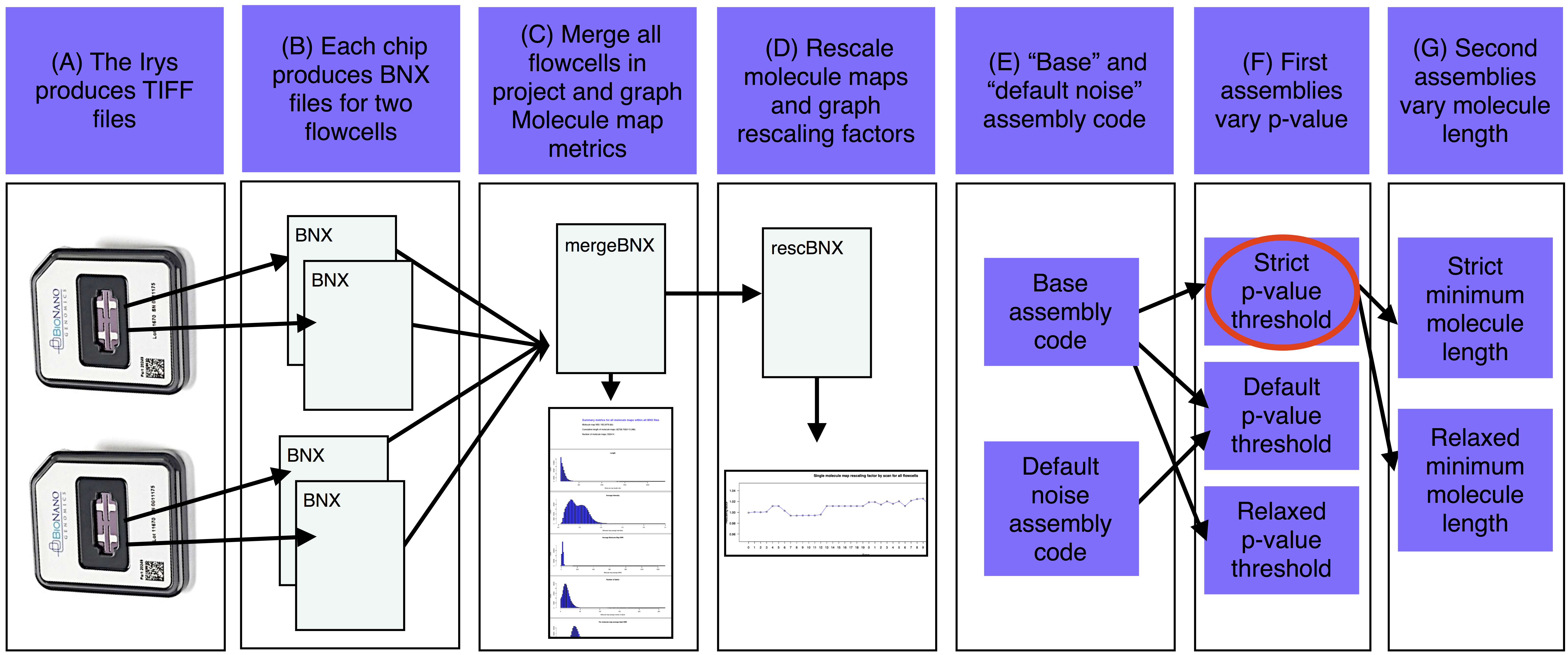
The basic steps of the assemble_XeonPhi pipeline are A) The Irys produces TIFF files that are converted into BNX text files of molecule maps. B) Each IrysChip produces one BNX file for each of two flowcells. C) Each BNX file in the bnx/ subdirectory of the -a assembly working directory is merged and molecule map quality metrics are summarized and plotted. D) If a reference is provided, merged BNX file is aligned to the in silico maps from the sequence reference. Stretch is rescaled from the alignment and the rescaling factor is ploted for each scan. Rescaled molecule maps are aligned to the reference and noise parameters are estimated. E) Base assembly code is determined based on estimated genome size and noise parameters. F) The first assemblies are run with a variety of p-value thresholds (at least one assembly is also run with defult noise parameters). G) The best of the first assemblies (red oval) is chosen and a version of this assembly is produced with a variety of minimum molecule length filters.
As you work through this lab your should read about the software are using by generating and reading the help menus.
Try the -man flag instead of the -help flag for a more detailed description of the program (you type q and enter to exit from a manual screen).
###Step 1: Clone the Git repositories
The following workflow requires that you install BioNano scripts and executables in ~/scripts and ~/tools directories respectively. Follow the Linux installation instructions in the "2.5.1 IrysSolve server RefAligner and Assembler" section of http://www.bnxinstall.com/training/docs/IrysViewSoftwareInstallationGuide.pdf.
When this is done install the KSU custom software using the code below:
cd ~
git clone https://github.com/i5K-KINBRE-script-share/Irys-scaffolding.git
git clone https://github.com/i5K-KINBRE-script-share/BNGCompare.git
###Step 2: Create project directory with sample input data in it
Make a working directory by making a copy of the sample_assembly_working_directory. This directory has a fragmented copy of the Escherichia coli str. K-12 substr. DH10B complete genome in it. While only the Molecules.bnx files have any content the file names listed are the same as the filenames one would see in an IrsyView workspace "Datasets" directory.
cp -r ~/Irys-scaffolding/KSU_bioinfo_lab/sample_assembly_working_directory ~
###Step 3: Check nick density
Read about the software in this section:
perl ~/Irys-scaffolding/KSU_bioinfo_lab/map_tools/nick_density.pl -help

perl ~/Irys-scaffolding/KSU_bioinfo_lab/assemble_XeonPhi/third-party/fa2cmap_multi.pl -help
In silico nick the genome FASTA and check nick density (to save time you can add the --two_enzyme flag to skip all but BspQI and BbvCI which are the two most commonly used enzymes if neither of these works re-run checking all possible enzymes)
perl ~/Irys-scaffolding/KSU_bioinfo_lab/map_tools/nick_density.pl ~/sample_assembly_working_directory/fasta_and_cmap/NC_010473_mock_scaffolds.fna
The goal is to find an enzyme or combination of enzymes that has between 10 and 20 nicks per 100 kb. In this case the results of nick_density.pl indicate that we should use the BspQI enzyme with an estimated 14.868 per 100 kb.
The nick_density.pl script created CMAPs for all possible enzymes that could be used for in silico map CMAPs or the labeling reaction. You can see these using the command below.
ls ~/sample_assembly_working_directory/fasta_and_cmap/cmaps/
If dual nicking (e.g. with BspQI and BbvCI) is required because single enzyme nick density is too low run the following command to create an in silico map CMAP.
perl ~/Irys-scaffolding/KSU_bioinfo_lab/assemble_XeonPhi/third-party/fa2cmap_multi.pl -v -i ~/sample_assembly_working_directory/fasta_and_cmap/NC_010473_mock_scaffolds.fna -e BspQI BbvCI
###Step 4: Get Molecules.bnx files from the IrysView Dataset subdirectories
Read about the software in this section:
perl ~/Irys-scaffolding/KSU_bioinfo_lab/assemble_XeonPhi/prep_bnxXeonPhi.pl -help
In a real workflow you will move the Datasets directory from IrysView to the assembly working directory and run prep_bnxXeonPhi.pl. In this case the Datasets directory is already in our assembly working directory.
perl ~/Irys-scaffolding/KSU_bioinfo_lab/assemble_XeonPhi/prep_bnxXeonPhi.pl -a ~/sample_assembly_working_directory
Check that this worked by looking for the Molecule BNX files in the new bnx subdirectory. The next scripts you call will assume any BNX file in the bnx sub directory of your assembly directory should be used in the assembly.
ls ~/sample_assembly_working_directory/bnx
#####Note, if you need to create a new Datasets directory for data directly from the Irys:
To create a new Datasets directory like this, run "AutoDetect" on your data. Next import the needed flowcells into a new IrsyView workspace. After importing you need to click on each flowcell listed in the workspace to generate a Molecules.bnx file from the RawMolecules.bnx file. After each click wait until the RunReport is displayed in IyrsView before moving to the next flowcell. Finally, move the entire Datasets directory to your linux machine and the same workflow as in this lab to analyze your own data.
###Step 5: Prepare molecule maps (i.e. maps in Molecules.bnx files) and write assembly scripts
Read about the software in this section:
perl ~/Irys-scaffolding/KSU_bioinfo_lab/assemble_XeonPhi/AssembleIrysXeonPhi.pl -help
Run AssembleIrysXeonPhi.pl to generate summary metrics for your molecule maps , MapStatsHistograms.pdf, and of the rescaling factors for each scan within a BNX file, bnx_rescaling_factors.pdf. Running AssembleIrysXeonPhi.pl will also output an assembly script named assembly_commands.sh that includes commands for assemblies with a variety of parameters. Each set of parameters has its own output sub directory created by the script.
perl ~/Irys-scaffolding/KSU_bioinfo_lab/assemble_XeonPhi/AssembleIrysXeonPhi.pl -a ~/sample_assembly_working_directory -g 5 -p Esch_coli_1_2015_000 -r ~/sample_assembly_working_directory/fasta_and_cmap/cmaps/NC_010473_mock_scaffolds_BspQI.cmap
Explore the output of this script in the ~/sample_assembly_working_directory/ directory.
The ~/sample_assembly_working_directory/Esch_coli_1_2015_000/MapStatsHistograms.pdf file contains information about the molecule maps > 100 kb. This information includes molecule map N50 and cumulative length, number of maps, molecule map signal-to-noise ratio (SNR), molecule map intensity, average label SNR per molecule map and average label intensity per molecule map.
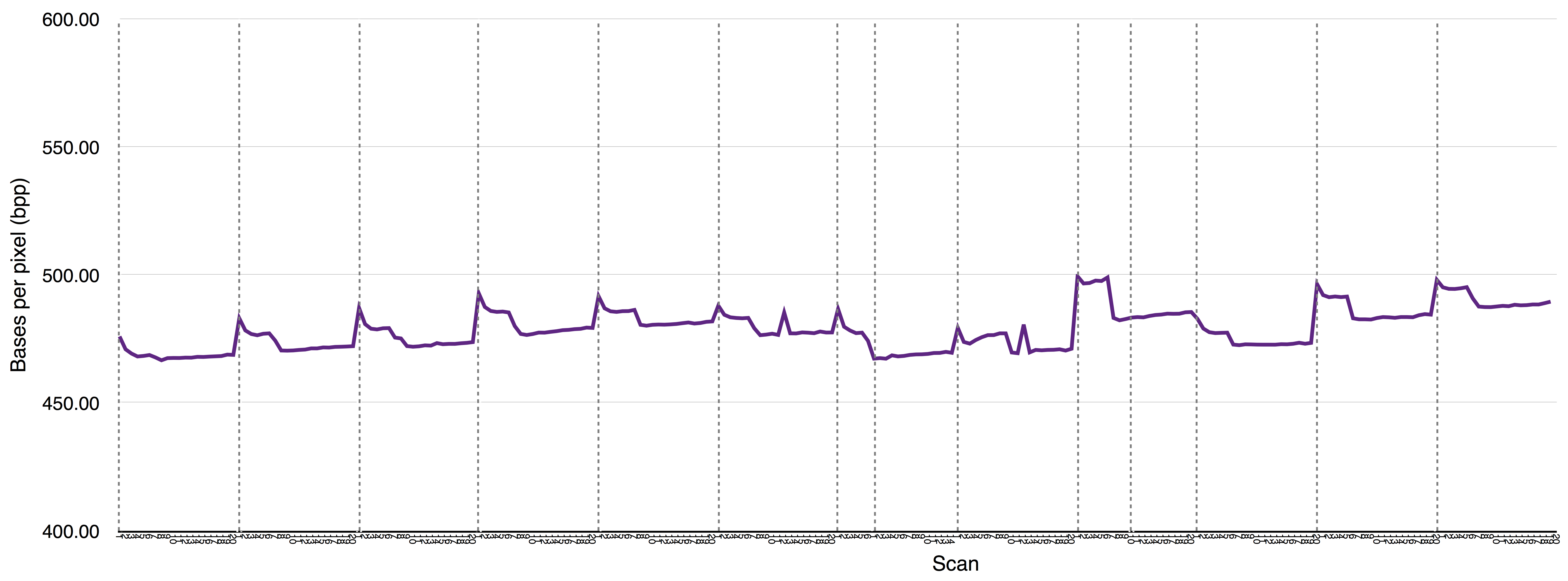
The ~/sample_assembly_working_directory/Esch_coli_1_2015_000/bnx_rescaling_factors.pdf file shows rescaling factors for each scan of a BNX file. This output will vary depending on the machine and IrysChip version used. It is also influenced by how similar the label motifs are between the samples runs on the Irys and the samples used to assembly the sequence-based reference. On your machine you may notice a predictable pattern for high quality BNX files. An example of one such a pattern is shown below:
The assembly script ~/sample_assembly_working_directory/assembly_commands.sh is written with all but four assembly commands commented out. If after running this command no satisfactory assemblies were created, uncomment assemblies with higher and/or lower minimum molecule map length and the best assembly p-value threshold. Also comment out the assemblies that have already run and save your script. Rerun the altered script to see if the new parameters improve the assembly.
###Step 6: Run assembly scripts
Read about the software in this section:
python2 ~/scripts/pipelineCL.py -help
Start your first four assemblies with the command below:
nohup bash ~/sample_assembly_working_directory/assembly_commands.sh &> ~/sample_assembly_working_directory/assembly_commands_out.txt
###Step 7: Evaluate your assemblies
Read about the software in this section:
perl ~/Irys-scaffolding/KSU_bioinfo_lab/assemble_XeonPhi/assembly_qcXeonPhi.pl -help
Check the quality of your assemblies with assembly_qcXeonPhi.pl.
perl ~/Irys-scaffolding/KSU_bioinfo_lab/assemble_XeonPhi/assembly_qcXeonPhi.pl -a ~/sample_assembly_working_directory -g 5 -p Esch_coli_1_2015_000
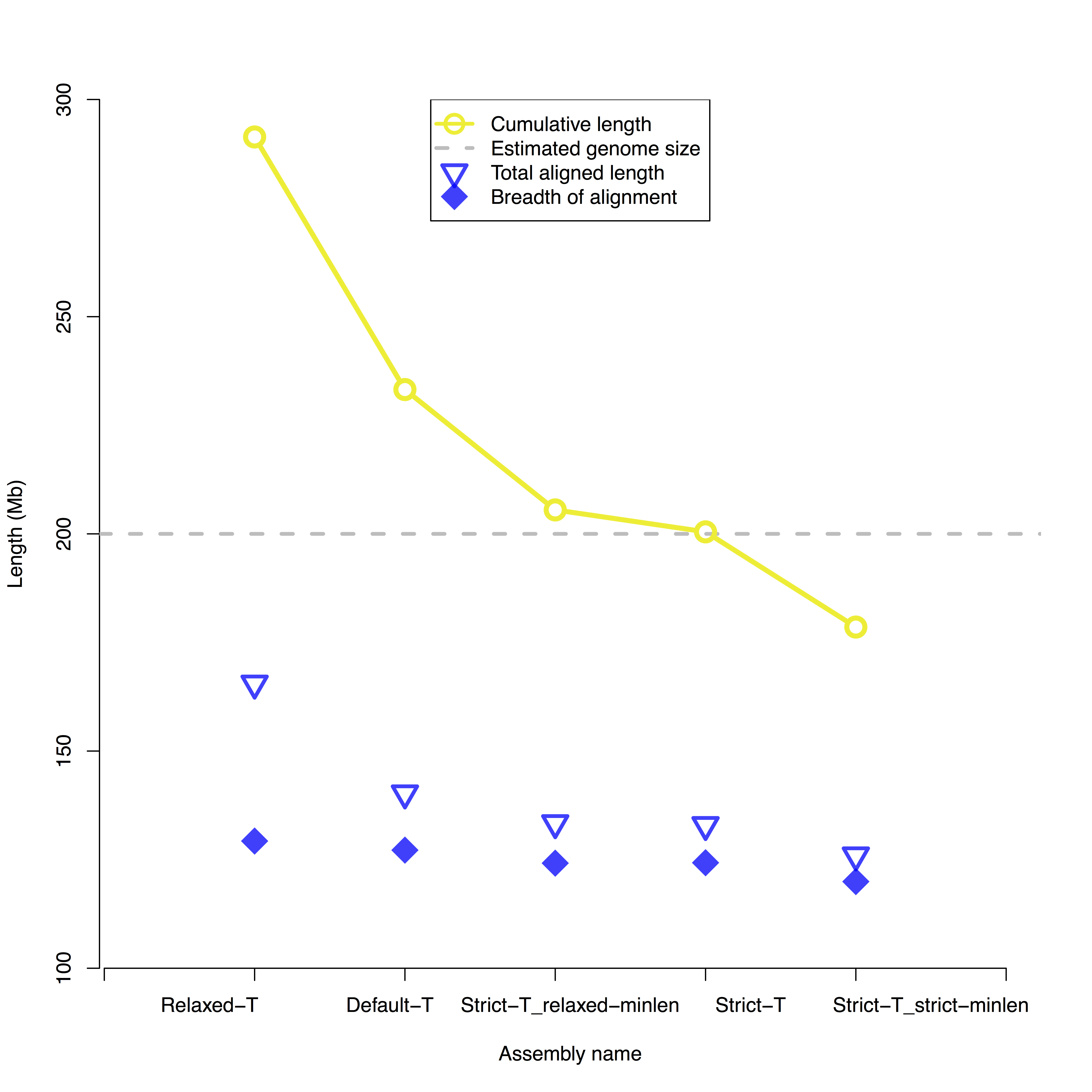
The ultimate goal is often to produce consensus genome maps that can be used to guide sequence-based haploid reference genome assembly. While single molecule maps can be used to reconstruct haplotypes, genome assembly involves collapsing polymorphisms arbitrarily into a consensus reference genome. Therefore the cumulative length of ideal consensus genome maps should equal the estimated haploid genome length. Additionally, 100% of the consensus genome maps would align non-redundantly to 100% of the in silico maps. In practice, the best BioNano assembly is selected based on similarity to the estimated haploid genome length and minimal alignment redundancy to the reference in silico maps. The greater the difference between "Breadth of alignment coverage" and "Length of total alignment" the greater the alignment redundancy.
For example, in the graph below the Strict-T assembly was the best of the assemblies because it has a cumulative size close to 200 Mb, the estimated size of that genome, and a small difference between non-redundant aligned length or "Breadth of alignment coverage", and the "Length of total alignment".
Take a look at the ~/sample_assembly_working_directory/Assembly_parameter_tests.pdf file to see the results for this assembly.
The file ~/sample_assembly_working_directory/Assembly_parameter_tests.csv has additional details about each assembly that can be used if there is no clear best assembly after reviewing ~/sample_assembly_working_directory/Assembly_parameter_tests.pdf.
###Step 8: Compare your best assembly to your reference in silico maps
Read about the software in this section:
perl ~/Irys-scaffolding/KSU_bioinfo_lab/stitch/sewing_machine.pl -help
sewing_machine.pl is a script that compiles assembly metrics and runs Stitch for the "best" assembly in all of the possible directories:'strict_t', 'default_t','relaxed_t', etc.
Stitch filters alignment XMAP files by confidence and the percent of the maximum potential length of the alignment. The first settings for confidence and the minimum percent of the full potential length of the alignment should be set to include the range that the researcher decides represent high quality alignments after viewing raw XMAPs. Some alignments have lower than optimal confidence scores because of low label density or short sequence-based scaffold length. The second set of filters should have a user-defined lower minimum confidence score, but a much higher percent of the maximum potential length of the alignment in order to capture these alignments. Resultant filtered XMAPs should be examined in IrysView to see that the alignments agree with what the user would manually select. Stitch finds the best super-scaffolding alignments each run. It is run iteratively by run_compare.pl until all super-scaffolds have been found.
We will start with the default filtering parameters for confidence scores (--f_con and --s_con) and percent of possible alignment thresholds (--f_algn and --s_algn). Generally we start with default parameters and then test more or less strict options if our first results are not satisfactory.
perl ~/Irys-scaffolding/KSU_bioinfo_lab/stitch/sewing_machine.pl -b ~/sample_assembly_working_directory/strict_t_150 -p Esch_coli_1_2015_000 -e BspQI -f ~/sample_assembly_working_directory/fasta_and_cmap/NC_010473_mock_scaffolds.fna -r ~/sample_assembly_working_directory/fasta_and_cmap/cmaps/NC_010473_mock_scaffolds_BspQI.cmap
###Step 9: Choose your best alignment parameters and summarize your results
Read about the software in this section:
perl ~/Irys-scaffolding/KSU_bioinfo_lab/assemble_XeonPhi/write_report.pl -help
Open the ~/sample_assembly_working_directory/NC_010473_mock_scaffolds_BNGCompare.csv file to find the best alignment parameters. Like choosing the best assembly you want to find a result that balances sensitivity (i.e. long total aligned length) without increasing alignment redundancy excessively.
perl ~/Irys-scaffolding/KSU_bioinfo_lab/assemble_XeonPhi/write_report.pl -b ~/sample_assembly_working_directory/strict_t_150 -p Esch_coli_1_2015_000 -e BspQI -f ~/sample_assembly_working_directory/fasta_and_cmap/NC_010473_mock_scaffolds.fna -r ~/sample_assembly_working_directory/fasta_and_cmap/cmaps/NC_010473_mock_scaffolds_BspQI.cmap --alignment_parameters default_alignment
###Step 10: Explore your results in IrysView
Read your ~/sample_assembly_working_directory/report.txt file or explore files in your ~/sample_assembly_working_directory/Esch_coli_1_2015_000 output directory. The contents of the ~/sample_assembly_working_directory/Esch_coli_1_2015_000 directory are also compressed in the ~/sample_assembly_working_directory/Esch_coli_1_2015_000.tar.gz file. Move this to a windows machine and follow instructions in the https://github.com/i5K-KINBRE-script-share/Irys-scaffolding/blob/master/KSU_bioinfo_lab/assemble_XeonPhi/README.pdf file to view alignments in IrysView. The following steps will be dificult to complete unless you have read the README.md file.
Following the instructions for loading an XMAP, first import the XMAP file of the alignment of the original in silico maps to the assembled genome maps. This will be in the Esch_coli_1_2015_000/align_in_silico_xmap directory.
Above is a screen shot of the first alignment (after ordering the anchors "in silico map #2", "in silico map #3", "in silico map #4", "in silico map #1").
Next import the XMAP file of the alignment of the super scaffolded in silico map to the assembled genome maps. This will be in the Esch_coli_1_2015_000/align_in_silico_super_scaffold_xmap directory.
Above is a screen shot of the second alignment (of the super scaffolded in silico map aligned to the genome maps).
Next load the BED file of the contigs for the super scaffolded in silico maps. This will be Esch_coli_1_2015_000/super_scaffold/Esch_coli_1_2015_000_20_40_15_90_2_superscaffold.fasta_contig.bed. There is also a BED file of the gaps for the super scaffolded in silico maps but the gaps for this sample genome are very small and therefore more difficult to view in the alignment Esch_coli_1_2015_000/super_scaffold/Esch_coli_1_2015_000_20_40_15_90_2_superscaffold.fasta_contig_gaps.bed.
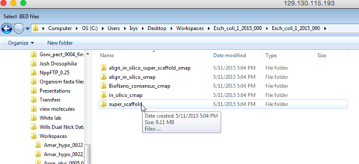
 Above is a screen shot of the menus that you will need to follow to begin to load the BED file.
 Above is a screen shot of the menus that you will need to follow to find the contig BED file for the super scaffolded in silico map.
 Above is a screen shot of the second alignment with the contig BED file loaded.
Switch from viewing the final superscaffold alignment. Load the the sv_xmap of the original in silico maps to the assembled genome maps from the smaps directory. You do this by highlighting the other alignment in the "Comparison Maps" window to the left. Follow the instructions in the README.md to import the SMAP and the merged BED files.
You will only see the annotation when viewing a single anchor from the "Anchor" drop down list at the bottom of the screen. Anchor #1 is the only anchor with predicted structural variants. Viewing the annotations will generally require redrawing the image according to the instructions in README.md.
 Above is a screenshot of the SV predictions for the in silico map anchor #1 after the SV annotation has loaded but before we have redrawn to view all labels.
 Above is a screenshot of the SV predictions for the in silico map anchor #1 after the SV annotation has loaded and after we have redrawn to view all labels.


