Copy relevant code from below to R/02_hello_keras.R and create a working model
Note how this is now a 3-class classifier and we are evaluating the predictive performance of the model on left out data.
The aim of this exercise is to let you build your first artificial
neural network using Keras. Naturally, we will use the iris data set.
library("tidyverse")
library("keras")The famous Iris flower data
set contains data
to quantify the morphologic variation of Iris flowers of three related
species. In other words - A total of 150 observations of 4 input
features Sepal.Length, Sepal.Width, Petal.Length and Petal.Width
and 3 output classes setosa versicolor and virginica, with 50
observations in each class:
iris %>% head## Sepal.Length Sepal.Width Petal.Length Petal.Width Species
## 1 5.1 3.5 1.4 0.2 setosa
## 2 4.9 3.0 1.4 0.2 setosa
## 3 4.7 3.2 1.3 0.2 setosa
## 4 4.6 3.1 1.5 0.2 setosa
## 5 5.0 3.6 1.4 0.2 setosa
## 6 5.4 3.9 1.7 0.4 setosa
Our aim is to create a model, which connect the 4 input features
(Sepal.Length, Sepal.Width, Petal.Length and Petal.Width) to the
correct output class (setosa versicolor and virginica) using an
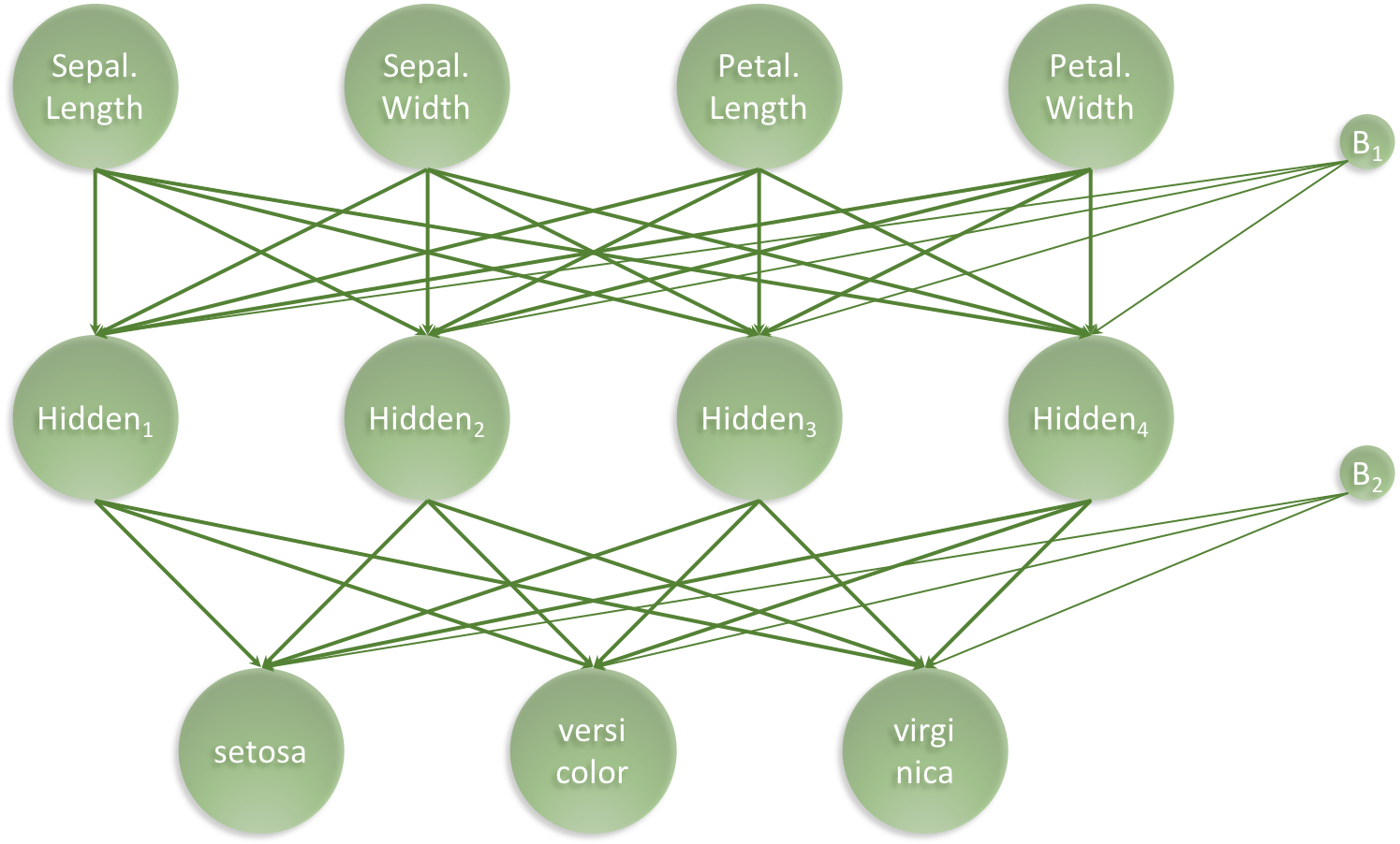
artificial neural network. For this task, we have chosen the following
simple architecture with one input layer with 4 neurons (one for each
feature), one hidden layer with 4 neurons and one output layer with 3
neurons (one for each class), all fully connected:
Our artificial neural network will have a total of 35 parameters: 4 for each input neuron connected to the hidden layer, plus an additional 4 for the associated first bias neuron and 3 for each of the hidden neurons connected to the output layer, plus an additional 3 for the associated second bias neuron. I.e. 4 x 4 + 4 + 4 x 3 + 3 = 35
We start with slightly wrangling the iris data set by renaming the input features and converting character labels to numeric:
nn_dat <- iris %>%
  as_tibble %>%
  rename(sepal_l_feat = Sepal.Length,
         sepal_w_feat = Sepal.Width,
         petal_l_feat = Petal.Length,
         petal_w_feat = Petal.Width) %>%
  mutate(class_num = as.numeric(Species) - 1, # factor, so = 0, 1, 2
         class_label = Species)
nn_dat %>%
  head(3)
## # A tibble: 3 x 7
## sepal_l_feat sepal_w_feat petal_l_feat petal_w_feat Species class_num
## <dbl> <dbl> <dbl> <dbl> <fct> <dbl>
## 1 5.1 3.5 1.4 0.2 setosa 0
## 2 4.9 3 1.4 0.2 setosa 0
## 3 4.7 3.2 1.3 0.2 setosa 0
## # … with 1 more variable: class_label <fct>
Then, we split the iris data into a training and a test data set, setting aside 20% of the data for left out data partition, to be used for final performance evaluation:
test_f <- 0.20
nn_dat <- nn_dat %>%
  mutate(partition = sample(x = c("train","test"),
                            size = nrow(.),
                            replace = TRUE,
                            prob = c(1 - test_f, test_f)))
nn_dat %>%
  count(partition)
## # A tibble: 2 x 2
## partition n
## <chr> <int>
## 1 test 43
## 2 train 107
Based on the partition, we can now create training and test data
# Training data
x_train <- nn_dat %>%
  filter(partition == "train") %>%
  select(contains("feat")) %>%
  as.matrix
y_train <- nn_dat %>%
  filter(partition == "train") %>%
  pull(class_num) %>%
  to_categorical(3)

# Test data
x_test <- nn_dat %>%
  filter(partition == "test") %>%
  select(contains("feat")) %>%
  as.matrix
y_test <- nn_dat %>%
  filter(partition == "test") %>%
  pull(class_num) %>%
to_categorical(3)Set architecture (See the green ANN visualisation)
model = keras_model_sequential() %>%
  layer_dense(units = 4, activation = "relu", input_shape = 4) %>%
  layer_dense(units = 3, activation = "softmax")
Compile model
model %>%
  compile(loss = "categorical_crossentropy",
          optimizer = optimizer_adam(),
          metrics = c("accuracy")
)
We can get a summary of the model like so:
model %>%
  summary
## Model: "sequential"
## ________________________________________________________________________________
## Layer (type) Output Shape Param #
## ================================================================================
## dense (Dense) (None, 4) 20
## ________________________________________________________________________________
## dense_1 (Dense) (None, 3) 15
## ================================================================================
## Total params: 35
## Trainable params: 35
## Non-trainable params: 0
## ________________________________________________________________________________
As expected we see 35 trainable parameters.
Lastly we fit the model and save the training progres in the history
object:
history <- model %>%
  fit(x = x_train,
      y = y_train,
      epochs = 200,
      batch_size = 16,
      validation_split = 0
)
Once the model is trained, we can inspect the training process
plot(history)## `geom_smooth()` using formula 'y ~ x'
The final performance can be obtained like so:
perf <- model %>%
  evaluate(x_test, y_test)
perf
## loss accuracy
## 0.2472026 0.9767442
Then we can augment the nn_dat for plotting:
plot_dat <- nn_dat %>%
  filter(partition == "test") %>%
  mutate(y_pred = predict_classes(model, x_test),
         Correct = ifelse(class_num == y_pred, "Yes", "No"))
plot_dat %>%
  select(-contains("feat")) %>%
  head(3)
## # A tibble: 3 x 6
## Species class_num class_label partition y_pred Correct
## <fct> <dbl> <fct> <chr> <dbl> <chr>
## 1 setosa 0 setosa test 0 Yes
## 2 setosa 0 setosa test 0 Yes
## 3 setosa 0 setosa test 0 Yes
and lastly, we can visualise the confusion matrix like so:
plot_dat %>%
  ggplot(aes(x = factor(y_pred),
             y = factor(class_num),
             colour = Correct)) +
  geom_jitter() +
  scale_x_discrete(labels = levels(nn_dat$class_label)) +
  scale_y_discrete(labels = levels(nn_dat$class_label)) +
  theme_bw() +
  labs(title = "Classification Performance of Artificial Neural Network",
       subtitle = str_c("Accuracy = ", round(perf["accuracy"], 3) * 100, "%"),
       x = "Predicted iris class",
y = "True iris class")Here, we created a 3-class predictor with an accuracy of 97.7% on a left
out data partition. I hope, this illustrates how relatively simple it is
to get started with Keras.


