Basic arithmetic, integration, differentiation, evaluation, and root finding over dense univariate polynomials.
(v1.5) pkg> add PolynomialsPolynomial– standard basis polynomials,a(x) = a₀ + a₁ x + a₂ x² + … + aₙ xⁿ,n ∈ ℕImmutablePolynomial– standard basis polynomials backed by a Tuple type for faster evaluation of valuesSparsePolynomial– standard basis polynomial backed by a dictionary to hold sparse high-degree polynomialsLaurentPolynomial– Laurent polynomials,a(x) = aₘ xᵐ + … + aₙ xⁿm ≤ n,m,n ∈ ℤbacked by an offset array; for example, ifm<0andn>0,a(x) = aₘ xᵐ + … + a₋₁ x⁻¹ + a₀ + a₁ x + … + aₙ xⁿChebyshevT– Chebyshev polynomials of the first kind
julia> using PolynomialsConstruct a polynomial from an array (a vector) of its coefficients, lowest order first.
julia> Polynomial([1,0,3,4])
Polynomial(1 + 3*x^2 + 4*x^3)
Optionally, the variable of the polynomial can be specified.
julia> Polynomial([1,2,3], :s)
Polynomial(1 + 2*s + 3*s^2)
Construct a polynomial from its roots.
julia> fromroots([1,2,3]) # (x-1)*(x-2)*(x-3)
Polynomial(-6 + 11*x - 6*x^2 + x^3)
Evaluate the polynomial p at x.
julia> p = Polynomial([1, 0, -1]);
julia> p(0.1)
0.99Methods are added to the usual arithmetic operators so that they work on polynomials, and combinations of polynomials and scalars.
julia> p = Polynomial([1,2])
Polynomial(1 + 2*x)

julia> q = Polynomial([1, 0, -1])
Polynomial(1 - x^2)

julia> p - q
Polynomial(2*x + x^2)

julia> p = Polynomial([1,2])
Polynomial(1 + 2*x)

julia> q = Polynomial([1, 0, -1])
Polynomial(1 - x^2)

julia> 2p
Polynomial(2 + 4*x)

julia> 2+p
Polynomial(3 + 2*x)

julia> p - q
Polynomial(2*x + x^2)

julia> p * q
Polynomial(1 + 2*x - x^2 - 2*x^3)

julia> q / 2
Polynomial(0.5 - 0.5*x^2)

julia> q ÷ p # `div`, also `rem` and `divrem`
Polynomial(0.25 - 0.5*x)
Operations involving polynomials with different variables will error.
julia> p = Polynomial([1, 2, 3], :x);
julia> q = Polynomial([1, 2, 3], :s);
julia> p + q
ERROR: Polynomials must have same variable.Integrate the polynomial p term by term, optionally adding a constant
term k. The degree of the resulting polynomial is one higher than the
degree of p (for a nonzero polynomial).
julia> integrate(Polynomial([1, 0, -1]))
Polynomial(1.0*x - 0.3333333333333333*x^3)

julia> integrate(Polynomial([1, 0, -1]), 2)
Polynomial(2.0 + 1.0*x - 0.3333333333333333*x^3)
Differentiate the polynomial p term by term. The degree of the
resulting polynomial is one lower than the degree of p.
julia> derivative(Polynomial([1, 3, -1]))
Polynomial(3 - 2*x)Return the roots (zeros) of p, with multiplicity. The number of
roots returned is equal to the degree of p. By design, this is not type-stable, the returned roots may be real or complex.
julia> roots(Polynomial([1, 0, -1]))
2-element Array{Float64,1}:
 -1.0
  1.0

julia> roots(Polynomial([1, 0, 1]))
2-element Array{Complex{Float64},1}:
 0.0 - 1.0im
 0.0 + 1.0im

julia> roots(Polynomial([0, 0, 1]))
2-element Array{Float64,1}:
 0.0
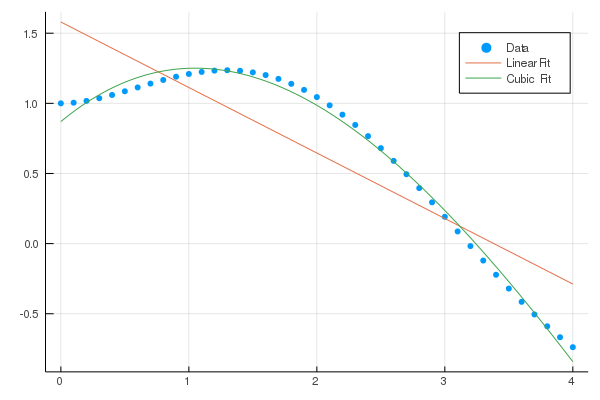
0.0Fit a polynomial (of degree deg or less) to x and y using a least-squares approximation.
julia> xs = 0:4; ys = @. exp(-xs) + sin(xs);

julia> fit(xs, ys) |> p -> round.(coeffs(p), digits=4) |> Polynomial
Polynomial(1.0 + 0.0593*x + 0.3959*x^2 - 0.2846*x^3 + 0.0387*x^4)

julia> fit(ChebyshevT, xs, ys, 2) |> p -> round.(coeffs(p), digits=4) |> ChebyshevT
ChebyshevT(0.5413⋅T_0(x) - 0.8991⋅T_1(x) - 0.4238⋅T_2(x))
Visual example:
Polynomial objects also have other methods:
-
0-based indexing is used to extract the coefficients of
[a0, a1, a2, ...], coefficients may be changed using indexing notation. -
coeffs: returns the entire coefficient vector -
degree: returns the polynomial degree,lengthis number of stored coefficients -
variable: returns the polynomial symbol as polynomial in the underlying type -
norm: find thep-norm of a polynomial -
conj: finds the conjugate of a polynomial over a complex field -
truncate: set to 0 all small terms in a polynomial; -
chopchops off any small leading values that may arise due to floating point operations. -
gcd: greatest common divisor of two polynomials. -
Pade: Return the Pade approximant of orderm/nfor a polynomial as aPadeobject.
-
StaticUnivariatePolynomials.jl Fixed-size univariate polynomials backed by a Tuple
-
MultiPoly.jl for sparse multivariate polynomials
-
DynamicPolynomals.jl Multivariate polynomials implementation of commutative and non-commutative variables
-
MultivariatePolynomials.jl for multivariate polynomials and moments of commutative or non-commutative variables
-
PolynomialRings A library for arithmetic and algebra with multi-variable polynomials.
-
AbstractAlgebra.jl, Nemo.jl for generic polynomial rings, matrix spaces, fraction fields, residue rings, power series, Hecke.jl for algebraic number theory.
-
CommutativeAlgebra the start of a computer algebra system specialized to discrete calculations with support for polynomials.
-
PolynomialRoots.jl for a fast complex polynomial root finder. For larger degree problems, also FastPolynomialRoots and AMRVW.
As of v0.7, the internals of this package were greatly generalized and new types and method names were introduced. For compatability purposes, legacy code can be run after issuing using Polynomials.PolyCompat.
If you are interested in contributing, feel free to open an issue or pull request to get started.

